An introduction to the SpatialFeatures Package
Guan Gui, Shila Ghazanfar
School of Mathematics and Statistics, The University of Sydney, Sydney, NSW, 2006, AustraliaCharles Perkins Centre, The University of Sydney, Sydney, NSW, 2006, AustraliaSydney Precision Data Science Centre, The University of Sydney, Sydney, NSW, 2006, AustraliaSource:
vignettes/SpatialFeatures.Rmd
SpatialFeatures.RmdSpatialFeatures
The R package SpatialFeatures contains functions to
extract features from molecule-resolved spatial transcriptomics data
using objects from the MoleculeExperiment class.
Load Required Libraries
library(SpatialFeatures)
library(MoleculeExperiment)
library(SingleCellExperiment)
library(ggplot2)
library(dplyr)
Create Example Dataset
Load an example MoleculeExperiment object with Xenium
data:
repoDir <- system.file("extdata", package = "MoleculeExperiment")
repoDir <- paste0(repoDir, "/xenium_V1_FF_Mouse_Brain")

me <- readXenium(repoDir, keepCols = "essential")
me
#> MoleculeExperiment class
#>
#> molecules slot (1): detected
#> - detected:
#> samples (2): sample1 sample2
#> -- sample1:
#> ---- features (137): 2010300C02Rik Acsbg1 ... Zfp536 Zfpm2
#> ---- molecules (962)
#> ---- location range: [4900,4919.98] x [6400.02,6420]
#> -- sample2:
#> ---- features (143): 2010300C02Rik Acsbg1 ... Zfp536 Zfpm2
#> ---- molecules (777)
#> ---- location range: [4900.01,4919.98] x [6400.16,6419.97]
#>
#>
#> boundaries slot (1): cell
#> - cell:
#> samples (2): sample1 sample2
#> -- sample1:
#> ---- segments (5): 67500 67512 67515 67521 67527
#> -- sample2:
#> ---- segments (9): 65043 65044 ... 65070 65071
Quick start
The spatialFeatures function performs three key steps.
First, it generates new boundaries corresponding to the feature types.
Second, it calculates entropy-based metrics for each of the feature
types. Third, it combines all this information and returns a
SingleCellExperiment object.
SpatialFeatures can be run with the following basic command. This will extract out all feature types as a single assay.
se = spatialFeatures(me)
se
#> class: SingleCellExperiment
#> dim: 178 14
#> metadata(0):
#> assays(4): subsector subconcentric supersector superconcentric
#> rownames(178): 2010300C02Rik Acsbg1 ... Zfp536 Zfpm2
#> rowData names(0):
#> colnames(14): sample1.67500 sample1.67512 ... sample2.65070
#>   sample2.65071
#> colData names(5): Cell Sample_id x_central y_central boundaries
#> reducedDimNames(0):
#> mainExpName: NULL
#> altExpNames(0):
You can also calculate gene counts within the spatialFeatures function, either as additional concatenated features, or with each feature type belonging to its own assay.
se = spatialFeatures(me, includeCounts = TRUE, concatenateFeatures = FALSE)
se
#> class: SingleCellExperiment
#> dim: 178 14
#> metadata(0):
#> assays(5): subsector subconcentric supersector superconcentric
#>   genecount
#> rownames(178): 2010300C02Rik Acsbg1 ... Zfp536 Zfpm2
#> rowData names(0):
#> colnames(14): sample1.67500 sample1.67512 ... sample2.65070
#>   sample2.65071
#> colData names(5): Cell Sample_id x_central y_central boundaries
#> reducedDimNames(0):
#> mainExpName: NULL
#> altExpNames(0):
Step-by-step SpatialFeatures
Generate new boundaries based on subcellular and supercellular features
This function loadBoundaries(me) processes the given
data (me) and returns feature data based on multiple assay
types, including: - Sub-Sector - Sub-Concentric - Super-Sector -
Super-Concentric
me <- SpatialFeatures::loadBoundaries(me)
me
#> MoleculeExperiment class
#>
#> molecules slot (1): detected
#> - detected:
#> samples (2): sample1 sample2
#> -- sample1:
#> ---- features (137): 2010300C02Rik Acsbg1 ... Zfp536 Zfpm2
#> ---- molecules (962)
#> ---- location range: [4900,4919.98] x [6400.02,6420]
#> -- sample2:
#> ---- features (143): 2010300C02Rik Acsbg1 ... Zfp536 Zfpm2
#> ---- molecules (777)
#> ---- location range: [4900.01,4919.98] x [6400.16,6419.97]
#>
#>
#> boundaries slot (5): cell subsector subconcentric supersector
#>   superconcentric
#> - cell:
#> samples (2): sample1 sample2
#> -- sample1:
#> ---- segments (5): 67500 67512 67515 67521 67527
#> -- sample2:
#> ---- segments (9): 65043 65044 ... 65070 65071
#> - subsector:
#> samples (2): sample1 sample2
#> -- sample1:
#> ---- segments (60): 67500_01 67500_02 ... 67527_11 67527_12
#> -- sample2:
#> ---- segments (108): 65043_01 65043_02 ... 65071_11 65071_12
#> - subconcentric:
#> samples (2): sample1 sample2
#> -- sample1:
#> ---- segments (30): 67500_01 67500_02 ... 67527_05 67527_06
#> -- sample2:
#> ---- segments (54): 65043_01 65043_02 ... 65071_05 65071_06
#> - supersector:
#> samples (2): sample1 sample2
#> -- sample1:
#> ---- segments (55): 67500_01 67500_02 ... 67527_10 67527_11
#> -- sample2:
#> ---- segments (99): 65043_01 65043_02 ... 65071_10 65071_11
#> - superconcentric:
#> samples (2): sample1 sample2
#> -- sample1:
#> ---- segments (35): 67500_01 67500_02 ... 67527_06 67527_07
#> -- sample2:
#> ---- segments (63): 65043_01 65043_02 ... 65071_06 65071_07
Draw the Feature Boundary Plots
Visualize the spatial molecule and cell boundary map with SpatialFeatures boundaries.
ggplot_me() +
  # add molecule points and colour by feature name
  geom_point_me(me, byColour = "feature_id", size = 0.1) +
  # add nuclei segments and colour the border with red
  geom_polygon_me(me, assayName = "subsector", fill = NA, colour = "red") +
  # add cell segments and colour by cell id
  geom_polygon_me(me, byFill = "segment_id", colour = "black", alpha = 0.1) +
  # zoom in to selected patch area
  coord_cartesian(xlim = c(4875, 4950), ylim = c(6385, 6455))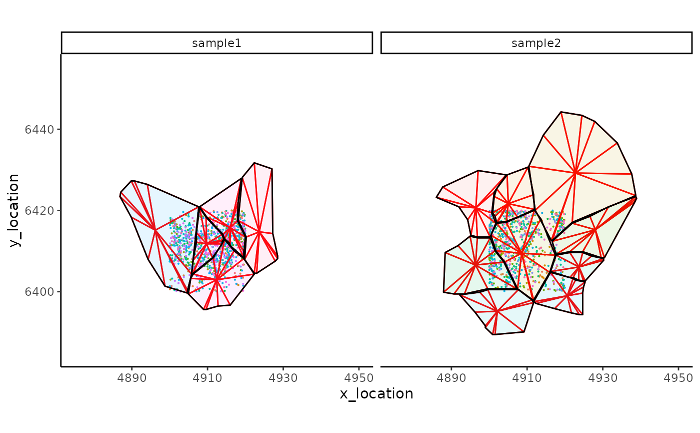
ggplot_me() +
  # add molecule points and colour by feature name
  geom_point_me(me, byColour = "feature_id", size = 0.1) +
  # add nuclei segments and colour the border with red
  geom_polygon_me(me, assayName = "subconcentric", fill = NA, colour = "red") +
  # add cell segments and colour by cell id
  geom_polygon_me(me, byFill = "segment_id", colour = "black", alpha = 0.1) +
  # zoom in to selected patch area
  coord_cartesian(xlim = c(4875, 4950), ylim = c(6385, 6455))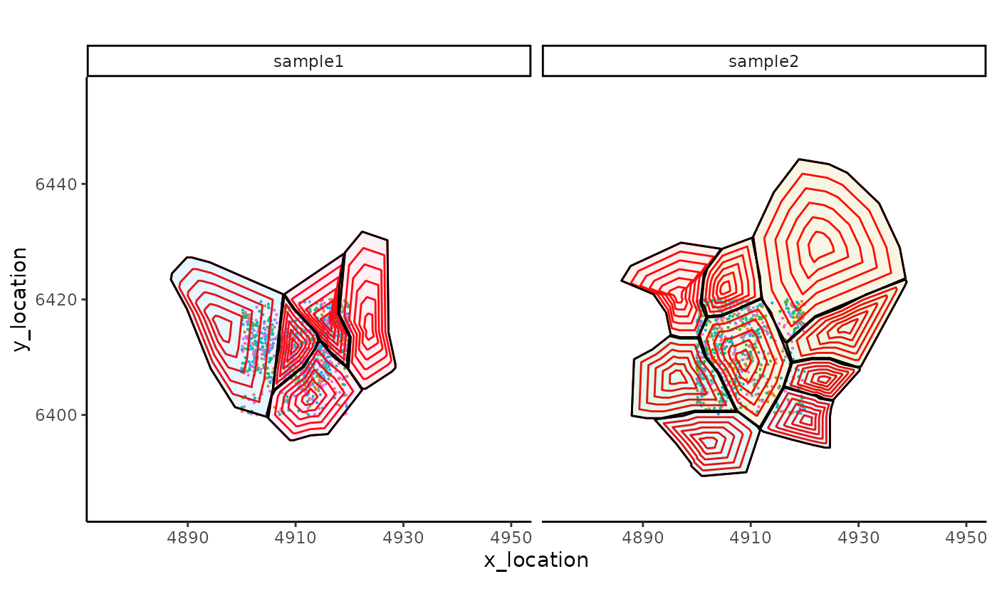
ggplot_me() +
  # add molecule points and colour by feature name
  geom_point_me(me, byColour = "feature_id", size = 0.1) +
  # add nuclei segments and colour the border with red
  geom_polygon_me(me, assayName = "supersector", fill = NA, colour = "blue") +
  # add cell segments and colour by cell id
  geom_polygon_me(me, byFill = "segment_id", colour = "black", alpha = 0.1) +
  # zoom in to selected patch area
  coord_cartesian(xlim = c(4875, 4950), ylim = c(6385, 6455))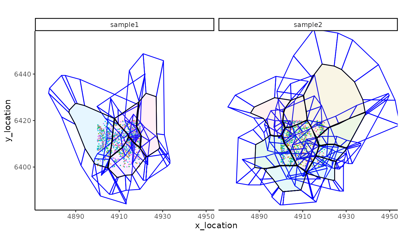
ggplot_me() +
  # add molecule points and colour by feature name
  geom_point_me(me, byColour = "feature_id", size = 0.1) +
  # add nuclei segments and colour the border with red
  geom_polygon_me(me, assayName = "superconcentric", fill = NA, colour = "blue") +
  # add cell segments and colour by cell id
  geom_polygon_me(me, byFill = "segment_id", colour = "black", alpha = 0.1) +
  # zoom in to selected patch area
  coord_cartesian(xlim = c(4875, 4950), ylim = c(6385, 6455))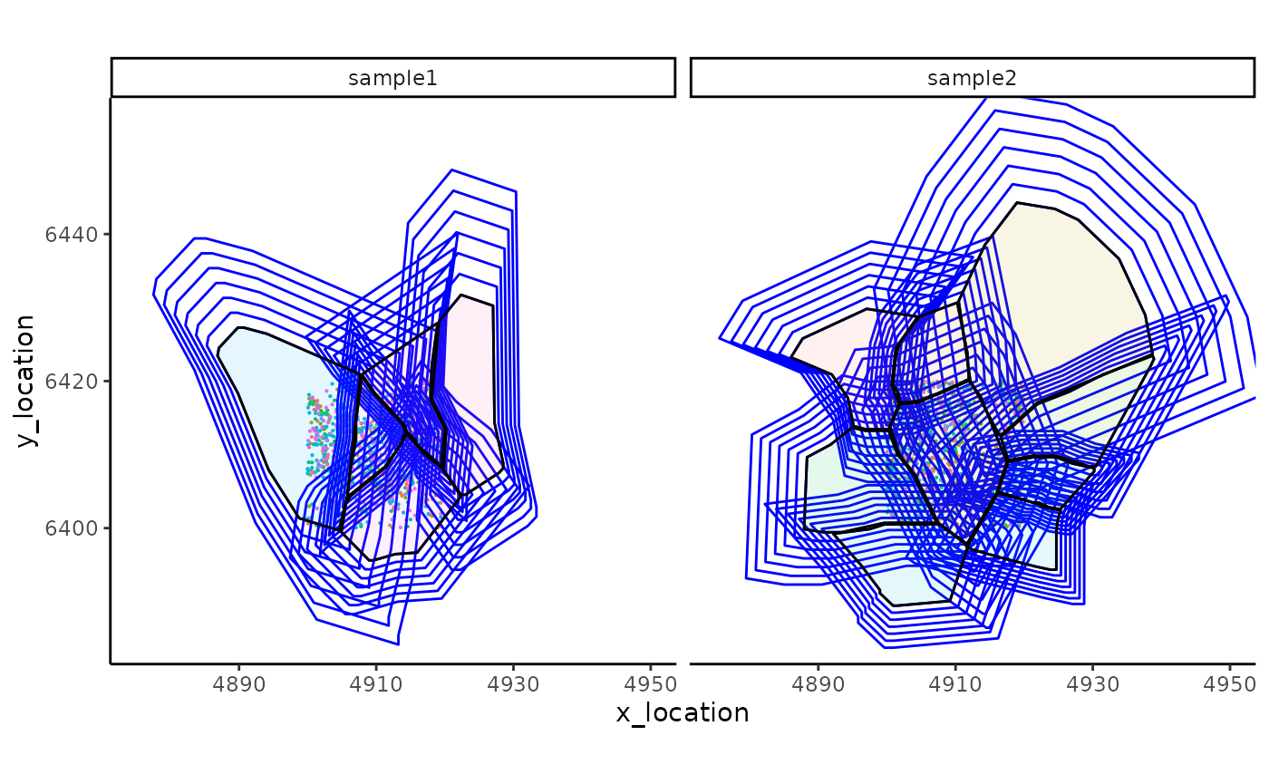
Create Entropy Matrix
This function EntropyMatrix() computes the entropy of a
counts matrix from a MoleculeExperiment object based on the
given assay type.
ent = SpatialFeatures::EntropyMatrix(me, c("subsector", "subconcentric", "supersector", "superconcentric"), nCores = 1)
lapply(ent, head, n = 4)
#> $subsector
#>               sample1.67500 sample1.67512 sample1.67515 sample1.67521
#> 2010300C02Rik     0.5623351     0.6931472     0.6365142     0.6931472
#> Acsbg1            0.6931472     0.6931472     0.6931472     0.0000000
#> Adamts2           0.0000000     0.0000000     0.0000000     0.0000000
#> Adamtsl1          0.0000000     0.0000000     0.0000000     0.0000000
#>               sample1.67527 sample2.65043 sample2.65044 sample2.65051
#> 2010300C02Rik             0             0             0     0.0000000
#> Acsbg1                    0             0             0     0.6931472
#> Adamts2                   0             0             0     0.0000000
#> Adamtsl1                  0             0             0     0.0000000
#>               sample2.65055 sample2.65063 sample2.65064 sample2.65067
#> 2010300C02Rik     1.5498260             0     0.6931472             0
#> Acsbg1            0.6931472             0     0.0000000             0
#> Adamts2           0.0000000             0     0.0000000             0
#> Adamtsl1          0.0000000             0     0.0000000             0
#>               sample2.65070 sample2.65071
#> 2010300C02Rik             0     0.0000000
#> Acsbg1                    0     0.6931472
#> Adamts2                   0     0.0000000
#> Adamtsl1                  0     0.0000000
#>
#> $subconcentric
#>               sample1.67500 sample1.67512 sample1.67515 sample1.67521
#> 2010300C02Rik     0.5623351     0.6931472     0.6365142             0
#> Acsbg1            0.6931472     0.0000000     0.6931472             0
#> Adamts2           0.0000000     0.0000000     0.0000000             0
#> Adamtsl1          0.0000000     0.0000000     0.0000000             0
#>               sample1.67527 sample2.65043 sample2.65044 sample2.65051
#> 2010300C02Rik             0             0             0             0
#> Acsbg1                    0             0             0             0
#> Adamts2                   0             0             0             0
#> Adamtsl1                  0             0             0             0
#>               sample2.65055 sample2.65063 sample2.65064 sample2.65067
#> 2010300C02Rik     1.2770343             0     0.6931472             0
#> Acsbg1            0.6931472             0     0.0000000             0
#> Adamts2           0.0000000             0     0.0000000             0
#> Adamtsl1          0.0000000             0     0.0000000             0
#>               sample2.65070 sample2.65071
#> 2010300C02Rik             0             0
#> Acsbg1                    0             0
#> Adamts2                   0             0
#> Adamtsl1                  0             0
#>
#> $supersector
#>               sample1.67500 sample1.67512 sample1.67515 sample1.67521
#> 2010300C02Rik             0      1.332179     0.6931472     0.6931472
#> Acsbg1                    0      0.000000     0.6931472     0.6931472
#> Adamts2                   0      0.000000     0.0000000     0.0000000
#> Adamtsl1                  0      0.000000     0.0000000     0.0000000
#>               sample1.67527 sample2.65043 sample2.65044 sample2.65051
#> 2010300C02Rik             0     0.5623351      1.039721     0.5982696
#> Acsbg1                    0     0.0000000      0.000000     0.9502705
#> Adamts2                   0     0.0000000      0.000000     0.0000000
#> Adamtsl1                  0     0.0000000      0.000000     0.0000000
#>               sample2.65055 sample2.65063 sample2.65064 sample2.65067
#> 2010300C02Rik      0.000000     0.6931472             0     0.0000000
#> Acsbg1             1.559581     1.0114043             0     0.6931472
#> Adamts2            0.000000     0.0000000             0     0.0000000
#> Adamtsl1           0.000000     0.0000000             0     0.0000000
#>               sample2.65070 sample2.65071
#> 2010300C02Rik     0.0000000     0.0000000
#> Acsbg1            0.5623351     0.6365142
#> Adamts2           0.0000000     0.0000000
#> Adamtsl1          0.0000000     0.0000000
#>
#> $superconcentric
#>               sample1.67500 sample1.67512 sample1.67515 sample1.67521
#> 2010300C02Rik     1.5607104       1.05492     0.6931472     0.0000000
#> Acsbg1            0.6931472       0.00000     0.6931472     0.6931472
#> Adamts2           0.0000000       0.00000     0.0000000     0.0000000
#> Adamtsl1          0.0000000       0.00000     0.0000000     0.0000000
#>               sample1.67527 sample2.65043 sample2.65044 sample2.65051
#> 2010300C02Rik     0.0000000      1.039721      1.386294      1.549826
#> Acsbg1            0.6931472      0.000000      0.000000      1.054920
#> Adamts2           0.0000000      0.000000      0.000000      0.000000
#> Adamtsl1          0.0000000      0.000000      0.000000      0.000000
#>               sample2.65055 sample2.65063 sample2.65064 sample2.65067
#> 2010300C02Rik     0.6931472     0.6931472      1.386294     0.0000000
#> Acsbg1            1.3208883     1.3296613      0.000000     0.6931472
#> Adamts2           0.0000000     0.0000000      0.000000     0.0000000
#> Adamtsl1          0.0000000     0.0000000      0.000000     0.0000000
#>               sample2.65070 sample2.65071
#> 2010300C02Rik     0.6931472     0.0000000
#> Acsbg1            0.6931472     0.6365142
#> Adamts2           0.0000000     0.0000000
#> Adamtsl1          0.0000000     0.0000000
Create SingleCellExperiment Object
This function EntropySingleCellExperiment() Convert the
entropy matrix into a SingleCellExperiment object.
se = SpatialFeatures::EntropySingleCellExperiment(ent, me)
se
#> class: SingleCellExperiment
#> dim: 178 14
#> metadata(0):
#> assays(4): subsector subconcentric supersector superconcentric
#> rownames(178): 2010300C02Rik Acsbg1 ... Zfp536 Zfpm2
#> rowData names(0):
#> colnames(14): sample1.67500 sample1.67512 ... sample2.65070
#>   sample2.65071
#> colData names(5): Cell Sample_id x_central y_central boundaries
#> reducedDimNames(0):
#> mainExpName: NULL
#> altExpNames(0):
If you also want the gene counts, you can include the parameter
se = EntropySingleCellExperiment(ent, me, includeCounts = TRUE)
se
#> class: SingleCellExperiment
#> dim: 178 14
#> metadata(0):
#> assays(5): subsector subconcentric supersector superconcentric
#>   genecount
#> rownames(178): 2010300C02Rik Acsbg1 ... Zfp536 Zfpm2
#> rowData names(0):
#> colnames(14): sample1.67500 sample1.67512 ... sample2.65070
#>   sample2.65071
#> colData names(5): Cell Sample_id x_central y_central boundaries
#> reducedDimNames(0):
#> mainExpName: NULL
#> altExpNames(0):
Inspect the SpatialFeatures SingleCellExperiment Object
Check the structure and content of the SingleCellExperiment object. This is a SingleCellExperiment with four assays corresponding to the different types of features that have been extracted.
se
#> class: SingleCellExperiment
#> dim: 178 14
#> metadata(0):
#> assays(5): subsector subconcentric supersector superconcentric
#>   genecount
#> rownames(178): 2010300C02Rik Acsbg1 ... Zfp536 Zfpm2
#> rowData names(0):
#> colnames(14): sample1.67500 sample1.67512 ... sample2.65070
#>   sample2.65071
#> colData names(5): Cell Sample_id x_central y_central boundaries
#> reducedDimNames(0):
#> mainExpName: NULL
#> altExpNames(0):
colData(se)
#> DataFrame with 14 rows and 5 columns
#>                        Cell   Sample_id x_central y_central
#>                 <character> <character> <numeric> <numeric>
#> sample1.67500 sample1.67500     sample1   4896.19   6415.14
#> sample1.67512 sample1.67512     sample1   4909.74   6411.80
#> sample1.67515 sample1.67515     sample1   4912.42   6402.93
#> sample1.67521 sample1.67521     sample1   4916.01   6415.75
#> sample1.67527 sample1.67527     sample1   4923.68   6414.74
#> ...                     ...         ...       ...       ...
#> sample2.65063 sample2.65063     sample2   4928.03   6415.25
#> sample2.65064 sample2.65064     sample2   4896.37   6406.56
#> sample2.65067 sample2.65067     sample2   4923.71   6406.08
#> sample2.65070 sample2.65070     sample2   4902.14   6395.17
#> sample2.65071 sample2.65071     sample2   4920.63   6398.99
#>                                                    boundaries
#>                                                        <AsIs>
#> sample1.67500 4896.85:6413.46,4895.15:6413.89,4894.30:6417.71
#> sample1.67512 4901.95:6417.07,4901.52:6418.56,4900.89:6419.41
#> sample1.67515 4916.40:6412.61,4912.15:6420.05,4910.45:6430.89
#> sample1.67521 4911.51:6397.95,4907.48:6400.71,4904.07:6407.30
#> sample1.67527 4929.57:6408.36,4924.69:6409.85,4921.29:6409.85
#> ...                                                       ...
#> sample2.65063 4904.71:6399.65,4898.76:6401.35,4894.30:6407.94
#> sample2.65064 4905.77:6404.11,4906.20:6407.73,4907.05:6412.19
#> sample2.65067 4908.96:6395.61,4904.93:6399.44,4905.56:6403.26
#> sample2.65070 4919.59:6408.36,4915.98:6411.34,4915.76:6411.98
#> sample2.65071 4922.35:6404.54,4919.80:6407.94,4920.23:6413.46
Alternatively, we could use the concatenateFeatures
argument to extract out all features as a single assay, as shown below.
In this case, the type of feature is recorded in the
rowData of the SingleCellExperiment
object.
se_concat = EntropySingleCellExperiment(ent, me,
                                        includeCounts = TRUE,
                                        concatenateFeatures = TRUE)
se_concat
#> class: SingleCellExperiment
#> dim: 890 14
#> metadata(0):
#> assays(1): spatialFeatures
#> rownames(890): subsector_2010300C02Rik subsector_Acsbg1 ...
#>   genecount_Zfp536 genecount_Zfpm2
#> rowData names(2): FeatureCategory FeatureGene
#> colnames(14): sample1.67500 sample1.67512 ... sample2.65070
#>   sample2.65071
#> colData names(5): Cell Sample_id x_central y_central boundaries
#> reducedDimNames(0):
#> mainExpName: NULL
#> altExpNames(0):
rowData(se_concat)
#> DataFrame with 890 rows and 2 columns
#>                         FeatureCategory   FeatureGene
#>                             <character>   <character>
#> subsector_2010300C02Rik       subsector 2010300C02Rik
#> subsector_Acsbg1              subsector        Acsbg1
#> subsector_Adamts2             subsector       Adamts2
#> subsector_Adamtsl1            subsector      Adamtsl1
#> subsector_Adgrl4              subsector        Adgrl4
#> ...                                 ...           ...
#> genecount_Vip                 genecount           Vip
#> genecount_Vwc2l               genecount         Vwc2l
#> genecount_Wfs1                genecount          Wfs1
#> genecount_Zfp536              genecount        Zfp536
#> genecount_Zfpm2               genecount         Zfpm2
Finish
sessionInfo()
#> R version 4.4.1 (2024-06-14)
#> Platform: x86_64-pc-linux-gnu
#> Running under: Ubuntu 22.04.5 LTS
#>
#> Matrix products: default
#> BLAS:   /usr/lib/x86_64-linux-gnu/openblas-pthread/libblas.so.3
#> LAPACK: /usr/lib/x86_64-linux-gnu/openblas-pthread/libopenblasp-r0.3.20.so;  LAPACK version 3.10.0
#>
#> locale:
#>  [1] LC_CTYPE=C.UTF-8       LC_NUMERIC=C           LC_TIME=C.UTF-8
#>  [4] LC_COLLATE=C.UTF-8     LC_MONETARY=C.UTF-8    LC_MESSAGES=C.UTF-8
#>  [7] LC_PAPER=C.UTF-8       LC_NAME=C              LC_ADDRESS=C
#> [10] LC_TELEPHONE=C         LC_MEASUREMENT=C.UTF-8 LC_IDENTIFICATION=C
#>
#> time zone: UTC
#> tzcode source: system (glibc)
#>
#> attached base packages:
#> [1] parallel  stats4    stats     graphics  grDevices utils     datasets
#> [8] methods   base
#>
#> other attached packages:
#>  [1] ggplot2_3.5.1               SpatialFeatures_0.99.1
#>  [3] purrr_1.0.2                 dplyr_1.1.4
#>  [5] SingleCellExperiment_1.26.0 SummarizedExperiment_1.34.0
#>  [7] Biobase_2.64.0              GenomicRanges_1.56.2
#>  [9] GenomeInfoDb_1.40.1         IRanges_2.38.1
#> [11] S4Vectors_0.42.1            BiocGenerics_0.50.0
#> [13] MatrixGenerics_1.16.0       matrixStats_1.4.1
#> [15] MoleculeExperiment_1.4.1    BiocStyle_2.32.1
#>
#> loaded via a namespace (and not attached):
#>  [1] tidyselect_1.2.1         EBImage_4.46.0           farver_2.1.2
#>  [4] bitops_1.0-9             fastmap_1.2.0            RCurl_1.98-1.16
#>  [7] digest_0.6.37            lifecycle_1.0.4          terra_1.7-83
#> [10] magrittr_2.0.3           compiler_4.4.1           rlang_1.1.4
#> [13] sass_0.4.9               tools_4.4.1              utf8_1.2.4
#> [16] yaml_2.3.10              data.table_1.16.2        knitr_1.48
#> [19] labeling_0.4.3           S4Arrays_1.4.1           htmlwidgets_1.6.4
#> [22] bit_4.5.0                DelayedArray_0.30.1      abind_1.4-8
#> [25] BiocParallel_1.38.0      withr_3.0.1              desc_1.4.3
#> [28] grid_4.4.1               fansi_1.0.6              colorspace_2.1-1
#> [31] scales_1.3.0             cli_3.6.3                rmarkdown_2.28
#> [34] crayon_1.5.3             ragg_1.3.3               generics_0.1.3
#> [37] httr_1.4.7               rjson_0.2.23             cachem_1.1.0
#> [40] zlibbioc_1.50.0          BiocManager_1.30.25      XVector_0.44.0
#> [43] tiff_0.1-12              vctrs_0.6.5              Matrix_1.7-0
#> [46] jsonlite_1.8.9           bookdown_0.41            fftwtools_0.9-11
#> [49] bit64_4.5.2              systemfonts_1.1.0        jpeg_0.1-10
#> [52] magick_2.8.5             locfit_1.5-9.10          jquerylib_0.1.4
#> [55] glue_1.8.0               pkgdown_2.1.1            codetools_0.2-20
#> [58] gtable_0.3.5             UCSC.utils_1.0.0         munsell_0.5.1
#> [61] tibble_3.2.1             pillar_1.9.0             htmltools_0.5.8.1
#> [64] GenomeInfoDbData_1.2.12  R6_2.5.1                 textshaping_0.4.0
#> [67] evaluate_1.0.1           lattice_0.22-6           highr_0.11
#> [70] png_0.1-8                SpatialExperiment_1.14.0 bslib_0.8.0
#> [73] Rcpp_1.0.13              SparseArray_1.4.8        xfun_0.48
#> [76] fs_1.6.4                 pkgconfig_2.0.3