Basic annotation pipeline#

This example creates a small spatial dataset, performs marker-priority tree gating, selects high-confidence labels, and visualises the result. It is executed from start to finish whenever the documentation is built.

Create an AnnData object#

For demonstration purposes, half the cells resemble T cells and half resemble B cells. Real data can be loaded from any source that produces an AnnData object with cells in rows and markers in columns.

import anndata as ad
import matplotlib.pyplot as plt
import numpy as np
import pandas as pd

import cytogater

rng = np.random.default_rng(42)
n_cells = 600
truth = np.repeat(["T cell", "B cell"], n_cells // 2)

expression = np.column_stack(
    [
        np.where(truth == "T cell", rng.normal(4, 0.7, n_cells), rng.normal(1, 0.5, n_cells)),
        np.where(truth == "B cell", rng.normal(4, 0.7, n_cells), rng.normal(1, 0.5, n_cells)),
    ]
)

adata = ad.AnnData(expression)
adata.var_names = ["CD3e", "CD20"]
adata.layers["exprs"] = expression.copy()
adata.obs["truth"] = pd.Categorical(truth)
adata.obsm["spatial"] = rng.uniform(0, 100, size=(n_cells, 2))
adata

AnnData object with n_obs × n_vars = 600 × 2
    obs: 'truth'
    obsm: 'spatial'
    layers: None (.X), 'exprs'

Define marker knowledge#

Positive markers support a cell-type assignment; negative markers penalise an assignment when they are expressed.

lineage_table = pd.DataFrame(
    {
        "cell_type": ["T cell", "B cell"],
        "pos_markers": [["CD3e"], ["CD20"]],
        "neg_markers": [["CD20"], ["CD3e"]],
    }
)
lineage_table

	cell_type	pos_markers	neg_markers
0	T cell	[CD3e]	[CD20]
1	B cell	[CD20]	[CD3e]

Run tree gating#

run_tree_gating() fits marker distributions, constructs a marker-priority tree for each cell type, and calculates a probability for every cell and cell type.

result = cytogater.run_tree_gating(
    adata,
    lineage_table,
    assay_name="exprs",
    min_cells=50,
    min_score=0.1,
    workers=1,
)

result["prob_mat"].head()

	T cell	B cell
0	0.286886	0.033399
1	0.228794	0.046117
2	0.299059	0.029000
3	0.303233	0.027430
4	0.174275	0.044564

The hard labels and probabilities are available both in the returned result and on the annotated object.

adata.obs[["truth", "cell_type_hard", "prob_best"]].head()

	truth	cell_type_hard	prob_best
0	T cell	T cell	0.286886
1	T cell	Uncertain	0.228794
2	T cell	T cell	0.299059
3	T cell	T cell	0.303233
4	T cell	Uncertain	0.174275

Select confident reference cells#

Probability cutoffs can identify an initial reference set for supervised prediction. Cells that do not uniquely exceed a cell-type cutoff remain Unknown.

result = cytogater.apply_cutoff_labels(result)
adata.obs["cutoff_label"].value_counts()

cutoff_label
Unknown    576
T cell      12
B cell      12
Name: count, dtype: int64

Inspect the spatial labels#

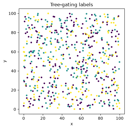
_images/6037c07d2a9579da08959e99c70a48734b116f507450657c0c765c61a4119cd5.png

The selected labels can now be used with cytogater.train_custom_knn(), cytogater.train_custom_randomforest(), or the hierarchical prediction workflow documented in the API reference.

Basic annotation pipeline

Contents