eNODAL
eNODAL.RmdIntroduction
Experimental guided nutriomics data clustering(eNODAL) method is an R package that facilitates discovery of relationships among high dimensional omics features and complex experimental condition.
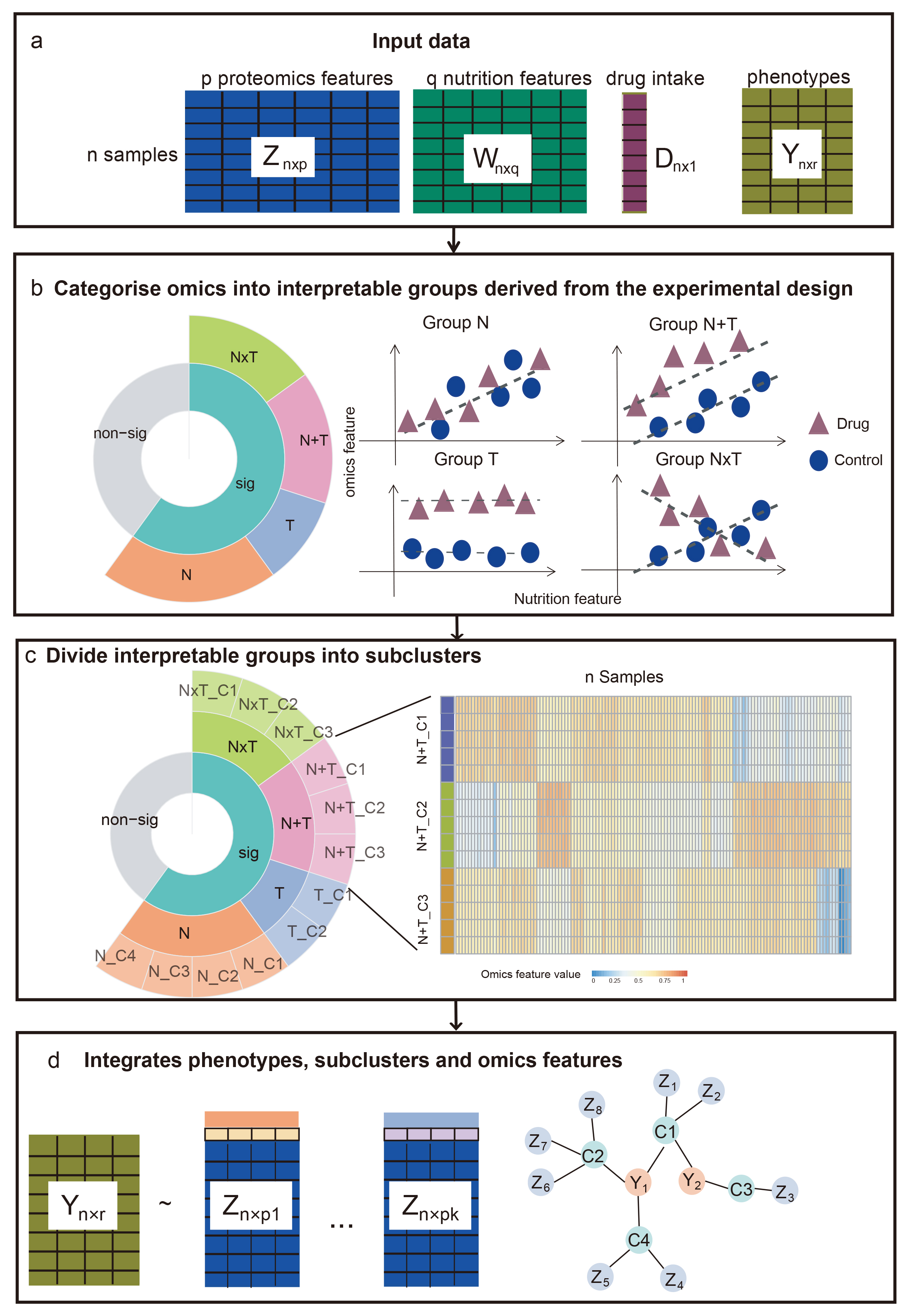
The method use a two-stage clustering method. At first stage, eNODAL using an ANOVA model to categorize omics features into several interpretable groups, in the second stage, eNODAL using consensus clustering method to further cluster each groups into sublcusters. The overall workflow of eNODAL shown in the following.
workflow
library(eNODAL)eNODAL use three modality as input, high dimensional omics features(Z), one set of experimental conditions, e.g. nutrition intake, denoted as Meta1 and another set of experimental conditions e.g. drug treatment, denoted as Meta2. Both of these factors can be (multiple) numerical variables or factors.
In this vignette, we go through a mouse liver proteomics data with different nutrition and drug treatment to analysis how nutrition and drug treatment influence these proteomics features.
Mouse liver proteomics data
The Proteomics dataset contain data from a mouse liver
proteomics study, the nutrition intake of each constructed from a
combination of 10 types of diet and the amount of food and nutrition is
measured. Each mouse takes one of four types of treatment, including
control, metformin, rapamycin and resveratrol, resulting 40 combinations
of complex experimental conditions
In this example, we simplified to first 1,000 proteomics and we will use eNODAL to categorize each proteomics feature interpretable group, significantly affected by 1) nutrition intake, 2) drug intake, 3) nutrition drug additive effect, 4) nutrition and drug interaction effect and 5) not signifcantly affected by all experimental conditions. Then eNODAL will further do consensus clustering for each interpretable group.
data("Proteomics")
Build the eNODAL object
First we build the eNODAL object, the input data to
build eNODAL have three part: omics data(Z), experimental
condition 1(Meta1) and experimental condition2(Meta2). (Meta1 and Meta2
better to be low dimensional). Meta1 and Meta2 can be both a vector or
dataframe. Z can be a matrix or dataframe. For all of these data, each
row is a sample and each column is a feature.
In the following example, we build eNODAL object based
on data in Proteomics.
Z <- Proteomics$Z
Meta1 <- Proteomics$Meta1
Meta2 <- Proteomics$Meta2
eNODAL object can also incorporate lots of parameters used in the
hypothesis testing, consensus clustering. Especially, we implemented
both linear model(lm) and general additive model(gam). Details of these
parameters see ?createParams. To accelerate the processing,
we use all linear model to for testing.
eNODAL_obj = eNODAL_build(Z = Z, Meta1 = Meta1, Meta2 = Meta2, sig_test = "lm", test_func = "lm")
Run the eNODAL.
Now using the runeNODAL function, we can run
eNODAL object with the specified parameters in the
eNODAL_build or createParams.
eNODAL_obj = runeNODAL(eNODAL_obj)which is equivalent to the following code
eNODAL_obj = runHT(eNODAL_obj) eNODAL_obj = runSubclust(eNODAL_obj)
The clustering result can be got by
Cl_df <- get_clusters(eNODAL_obj)And the resulting cluster can be shown by
show_clusters(eNODAL_obj)
#> Level0, significant vs. non-significant under experimental condition:
#>  non-sig(196), sig(804)
#> Level1, marginal effect vs. interaction effect:
#>  Add(278), Int(181), Meta1(342), Meta2(3)
#> Level2, unsupervised clustering within each cluster:
#>  Add_C1(39), Add_C2(52), Add_C3(23), Add_C4(16), Add_C5(63), Add_C6(25), Add_C7(9), Add_C8(28), Add_C9(23), Int_C1(28), Int_C2(24), Int_C3(49), Int_C4(22), Int_C5(18), Int_C6(20), Int_C7(20), Meta1_C1(65), Meta1_C10(15), Meta1_C2(72), Meta1_C3(13), Meta1_C4(36), Meta1_C5(25), Meta1_C6(29), Meta1_C7(37), Meta1_C8(31), Meta1_C9(19), Meta2_C1(3)
and can also be visualized by
ClusterPlot(eNODAL_obj)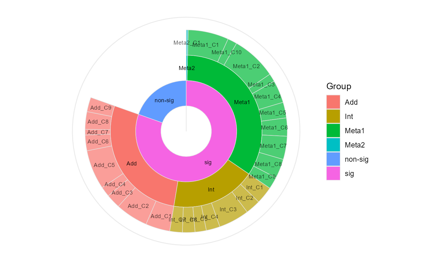
Visualization
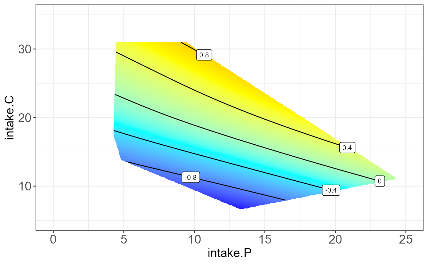
In this section, we will show how to visualize relationships between omics feautures, (or resulting cluters) and continuous variables(nutrition intake) by nutrition geometry framewor and discrete variables(drug intake) by boxplot.
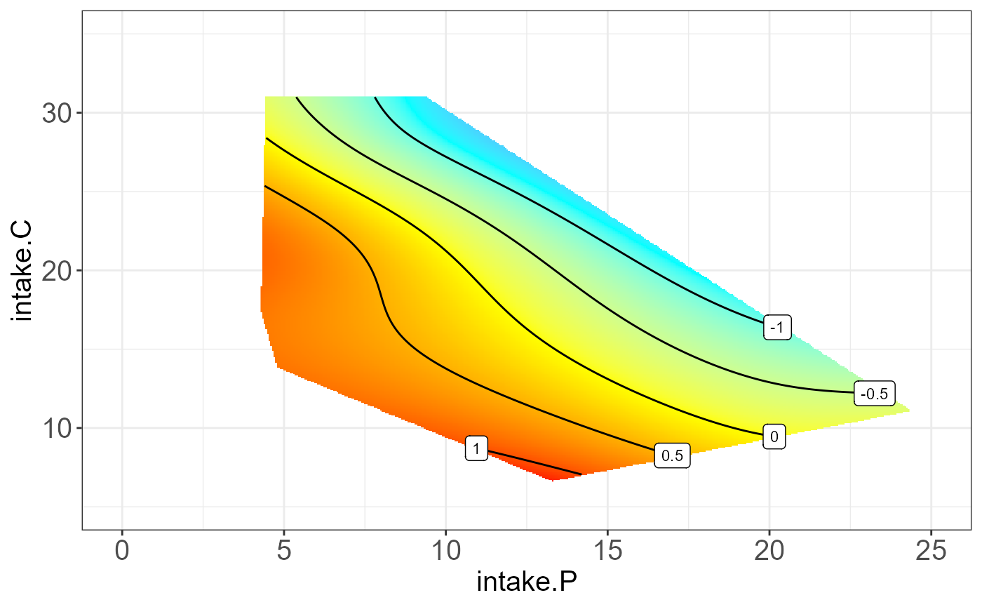
Nutrition geometry framework(NGF)
Even we do not do runeNODAL, we can also run NGF based
on selected omics features (can be both feature name or index). In the
following example, we will illustrate the NGF of eNODAL object on
protein P19096 on “intake.P”, “intake.C” and “intake.F”.
The resulting NGF will be any two combination of nutrition feature and
the third one be the median.
#>
#> [[2]]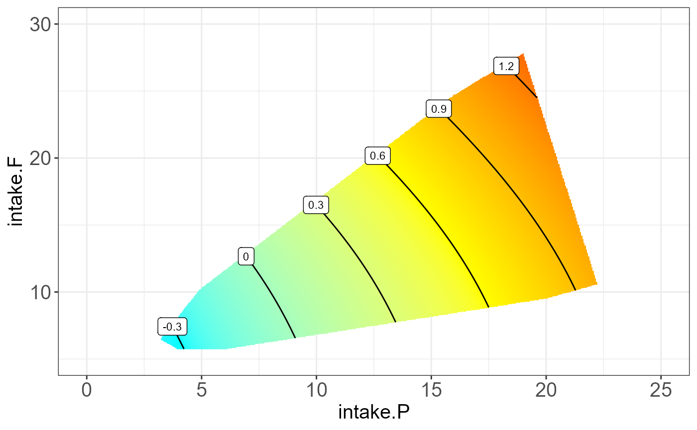
#>
#> [[3]]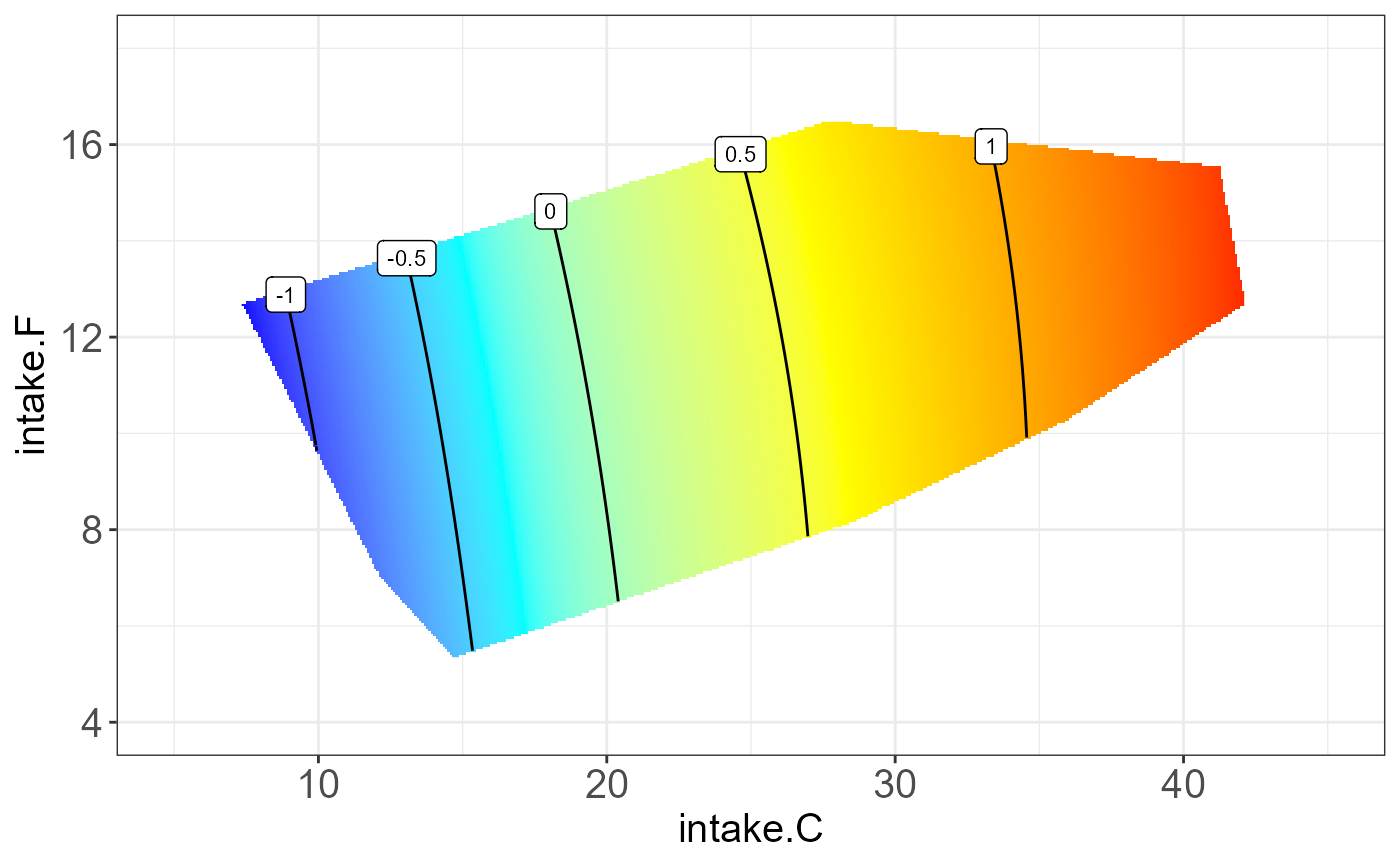
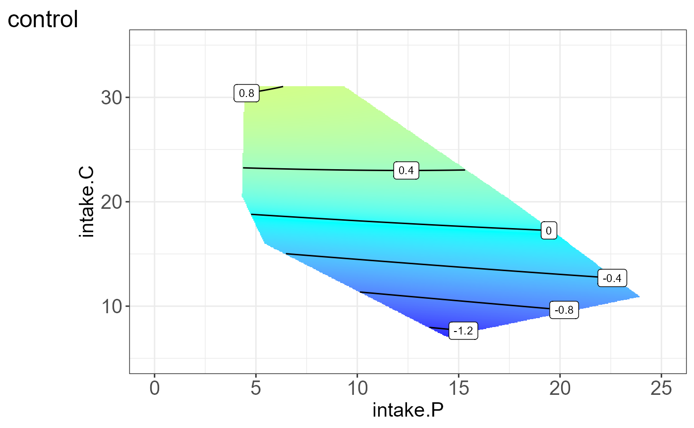
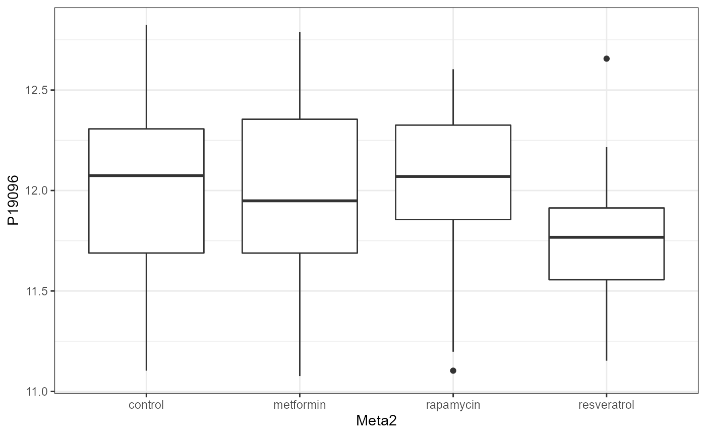
We can also visualize the protein for each group, i.e. split by “Meta2”(Drug) and the resulting NGF are shown below.
#>
#> [[2]]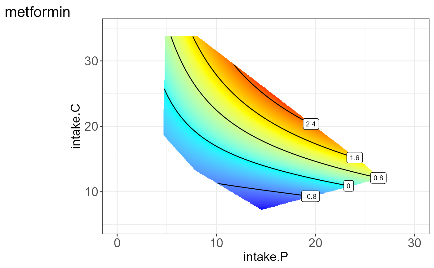
#>
#> [[3]]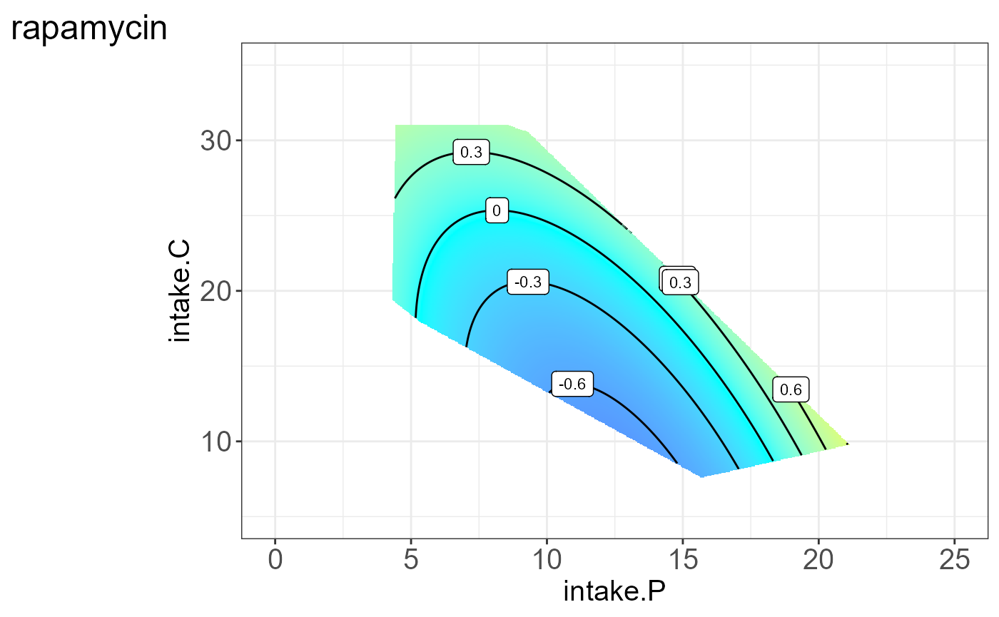
#>
#> [[4]]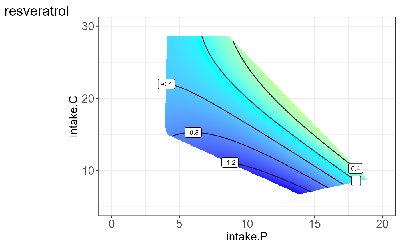
#>
#> [[5]]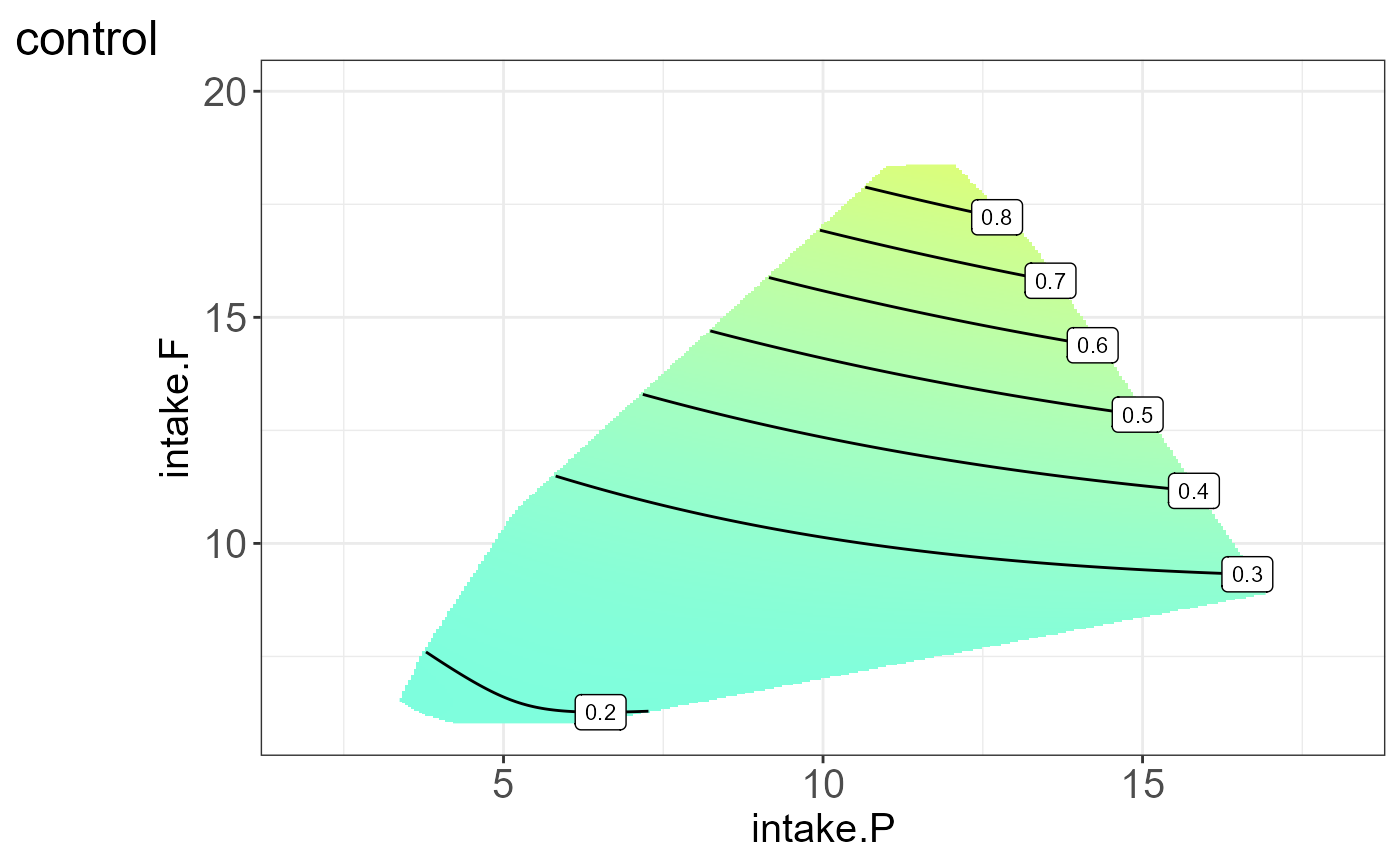
#>
#> [[6]]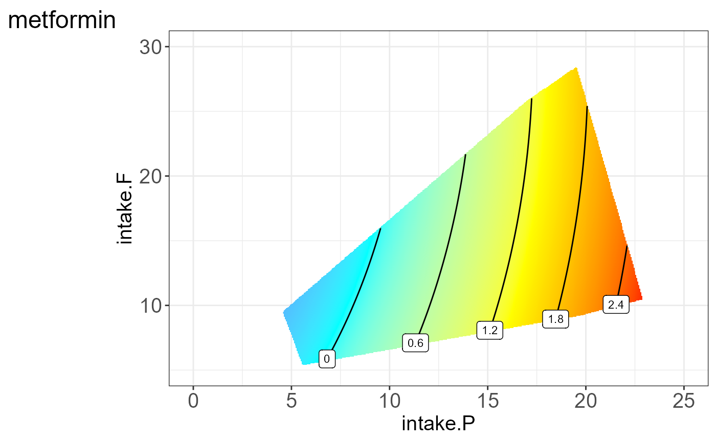
#>
#> [[7]]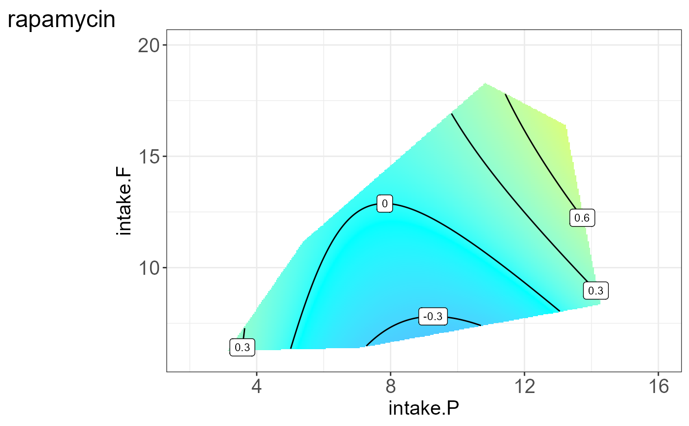
#>
#> [[8]]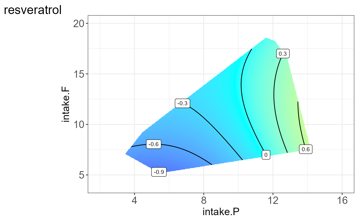
#>
#> [[9]]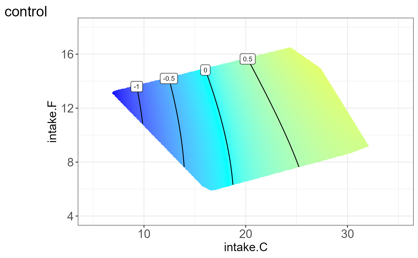
#>
#> [[10]]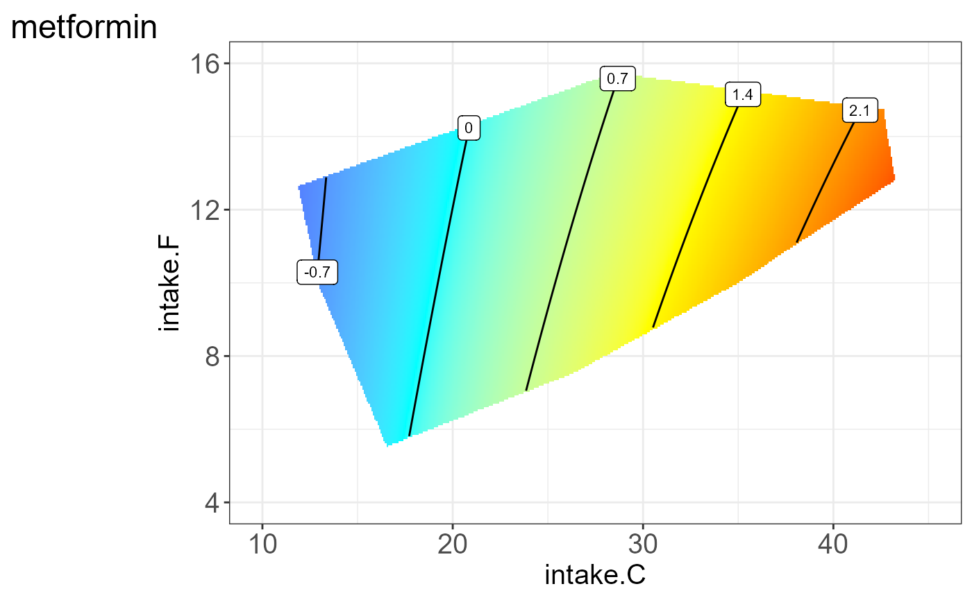
#>
#> [[11]]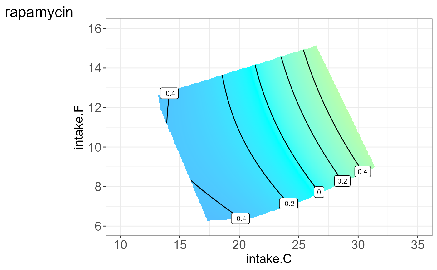
#>
#> [[12]]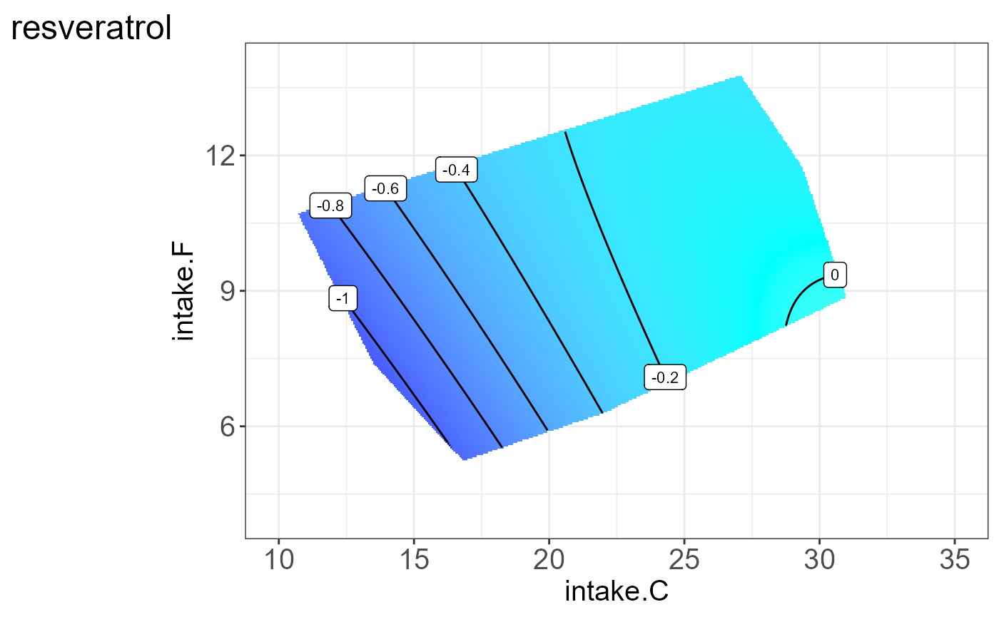 We can also visualize the interpretable groups or subclusters by their
first principal component.
We can also visualize the interpretable groups or subclusters by their
first principal component.
#>
#> [[2]]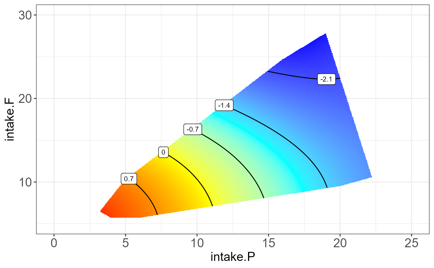
#>
#> [[3]]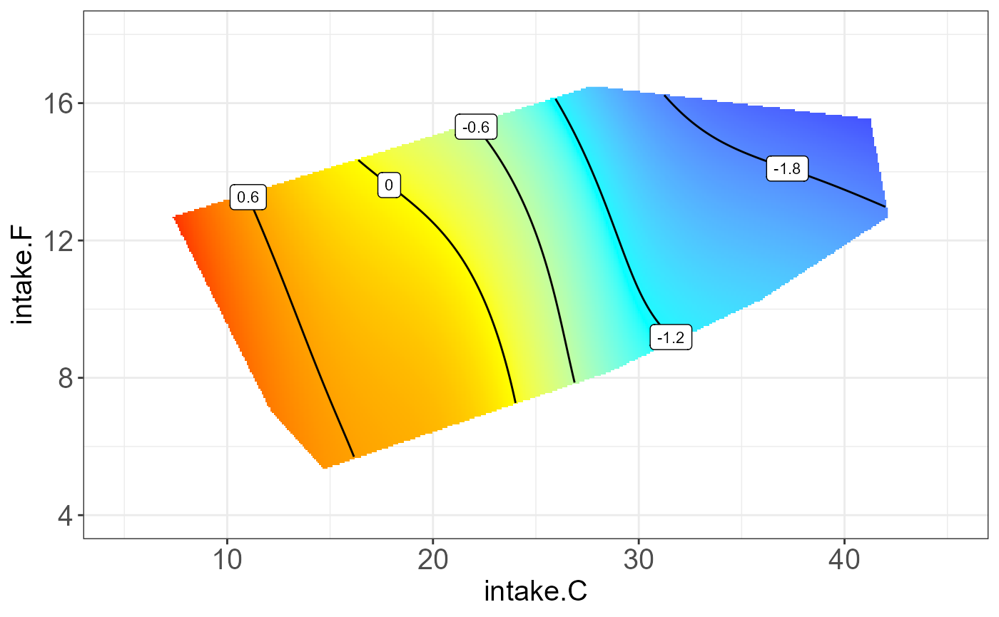
Misc
sessionInfo()
#> R version 4.1.0 (2021-05-18)
#> Platform: x86_64-w64-mingw32/x64 (64-bit)
#> Running under: Windows 10 x64 (build 22000)
#>
#> Matrix products: default
#>
#> locale:
#> [1] LC_COLLATE=Chinese (Simplified)_China.936
#> [2] LC_CTYPE=Chinese (Simplified)_China.936
#> [3] LC_MONETARY=Chinese (Simplified)_China.936
#> [4] LC_NUMERIC=C
#> [5] LC_TIME=Chinese (Simplified)_China.936
#>
#> attached base packages:
#> [1] stats     graphics  grDevices utils     datasets  methods   base
#>
#> other attached packages:
#> [1] eNODAL_0.1.0
#>
#> loaded via a namespace (and not attached):
#>  [1] Rcpp_1.0.7          lubridate_1.7.10    lattice_0.20-44
#>  [4] assertthat_0.2.1    rprojroot_2.0.2     digest_0.6.27
#>  [7] utf8_1.2.2          plyr_1.8.6          R6_2.5.1
#> [10] backports_1.2.1     magic_1.6-0         stats4_4.1.0
#> [13] evaluate_0.15       ggplot2_3.3.6       highr_0.9
#> [16] pillar_1.8.1        rlang_1.0.4         data.table_1.14.0
#> [19] rstudioapi_0.13     jquerylib_0.1.4     S4Vectors_0.30.0
#> [22] Matrix_1.3-4        checkmate_2.0.0     rmarkdown_2.10
#> [25] apcluster_1.4.10    pkgdown_1.6.1       labeling_0.4.2
#> [28] textshaping_0.3.5   desc_1.3.0          splines_4.1.0
#> [31] stringr_1.4.0       igraph_1.2.6        munsell_0.5.0
#> [34] metR_0.12.0         compiler_4.1.0      xfun_0.30
#> [37] pkgconfig_2.0.3     systemfonts_1.0.2   BiocGenerics_0.38.0
#> [40] mgcv_1.8-36         htmltools_0.5.2     tidyselect_1.1.1
#> [43] tibble_3.1.8        fansi_1.0.3         crayon_1.5.1
#> [46] dplyr_1.0.7         MASS_7.3-54         grid_4.1.0
#> [49] nlme_3.1-153        jsonlite_1.7.2      gtable_0.3.0
#> [52] lifecycle_1.0.1     DBI_1.1.3           magrittr_2.0.3
#> [55] scales_1.2.1        cli_3.0.1           stringi_1.7.4
#> [58] cachem_1.0.6        farver_2.1.1        fs_1.5.0
#> [61] geometry_0.4.5      bslib_0.3.0         ragg_1.1.3
#> [64] generics_0.1.3      vctrs_0.4.1         tools_4.1.0
#> [67] glue_1.6.2          purrr_0.3.4         abind_1.4-5
#> [70] parallel_4.1.0      fastmap_1.1.0       yaml_2.2.1
#> [73] colorspace_2.0-2    isoband_0.2.5       memoise_2.0.1
#> [76] knitr_1.38          sass_0.4.0