2 Evaluation using Trio
Source:vignettes/v02_Evaluation_using_Trio.Rmd
v02_Evaluation_using_Trio.RmdImport microbiome data
The Trio object in BenchHub can take
datasets provided by users. To demonstrate this workflow, we use the
lubomski_microbiome_data example dataset distributed with
BenchHub. We first load the example objects into a
temporary environment to avoid placing x and
lubomPD directly into the global workspace. The dataset
contains two objects: x, a 575 by 1192 matrix of microbial
abundances for 575 samples, and lubomPD, a binary factor
indicating Parkinson’s disease (PD) or healthy control
(HC) status for each sample.
# import the microbiome data into a temporary environment
exampleEnv <- new.env(parent = emptyenv())
data("lubomski_microbiome_data", envir = exampleEnv, package = "BenchHub")

x <- exampleEnv[["x"]]
lubomPD <- exampleEnv[["lubomPD"]]

# check the dimension of the microbiome matrix
dim(x)
## [1] 575 1192
# check the length of the patient status
length(lubomPD)
## [1] 575The task we’ll be evaluating uses a binary classification task where
each sample is either a Parkinson’s Disease (PD) patient or Healthy
Control (HC). Once the data are ready to be inputted to
Trio, we can load Trio.
Initialise a Trio object
To initialise a Trio object, we use a new() method.
trio <- Trio$new(data = x,
                 evidence = list(
                   Diagnosis = list(
                     evidence = lubomPD,
                     metrics = "Balanced Accuracy"
                     )
                   ),
                 metrics = list(
                   `Balanced Accuracy` = balAccMetric
                   ),
                 datasetID = "lubomski_microbiome"
                 )
The supporting evidence is the disease diagnosis, which is the
lubomPD vector that we extracted from the
Lubomski data above and the relevant metric to evaluate it
is Balanced Accuracy. Next, we will use this microbiome data to
illustrate two examples, 1) evaluation with cross validation, 2)
evaluation without cross validation.
Cross validation - using the trio split function
In this example, we show a typical classification scenario to classify the patient status, where we need to split the data into training and testing set.
Step 1: Obtain relevant data for the model. To build a model, the
following code will extract the data matrix and patient status outcome
from Trio object.
# get the gold standard from the Trio object
x <- trio$data
y <- trio$getEvidence("Diagnosis")
Step 2: For repeated cross-validation, the split()
function will split the y vector (i.e.,
evidence) into the number of folds and repeats users want.
In this case we used n_fold = 2 and
n_repeat = 5 (i.e., 2-fold cross-validation with 10
repeats). Then users can get cross-validation indices
(CVindices) for each sample, through
splitIndices. This gives a simple list where each element
represents a combination of folds and repeats for each sample.
# get train and test indices
trio$split(y = y, n_fold = 2, n_repeat = 5)
CVindices <- trio$splitIndices
Step 5: Build the classification model and evaluate. We can now use a for loop to cross-validate evaluation results.
Using the CVindices, user can subset to training and
test data. As an example, we build a LASSO regression model as a
classification model on the training data, then make predictions on the
test data.
Once predictions are obtained for the test set, we pass them to Trio
using the same evidence name as stored in the Trio object (i.e.,
Diagnosis). Specifically, we call
trio$evaluate(list(lasso = list(Diagnosis = pred))), which
instructs evaluate() to compare pred against
the reference labels Diagnosis stored in trio,
and then compute the specified metric (Balanced Accuracy).
We first construct an explicit cross-validation plan that records fold and repeat identifiers, and then iterate over this plan to evaluate each split.
set.seed(1234)
library(tibble)

cv_plan <- tibble(
  trainIDs = CVindices,
  fold = vapply(
    strsplit(names(CVindices), ".", fixed = TRUE),
    `[`,
    character(1),
    1
  ),
  repeat_id = vapply(
    strsplit(names(CVindices), ".", fixed = TRUE),
    `[`,
    character(1),
    2
  )
)

run_one_cv <- function(trainIDs, fold, repeat_id, trio, x, y) {
  x_train <- x[trainIDs, ]
  x_test  <- x[-trainIDs, ]
  y_train <- y[trainIDs]
  y_test  <- y[-trainIDs]

  cv_lasso <- glmnet::cv.glmnet(
    x = as.matrix(x_train),
    y = y_train,
    alpha = 1,
    family = "binomial"
  )
  lam <- cv_lasso$lambda.1se

  fit <- glmnet::glmnet(
    x = as.matrix(x_train),
    y = y_train,
    alpha = 1,
    lambda = lam,
    family = "binomial"
  )

  pred <- predict(
    fit,
    newx = as.matrix(x_test),
    s = lam,
    type = "class"
  )
  pred <- setNames(as.factor(as.vector(pred)), rownames(x_test))

  eval_res <- trio$evaluate(list(lasso = list(Diagnosis = pred)))

  # attach metadata explicitly
  eval_res$fold <- fold
  eval_res$repeat_id <- repeat_id

  eval_res
}

result_list <- vector("list", nrow(cv_plan))

for (i in seq_len(nrow(cv_plan))) {
  result_list[[i]] <- run_one_cv(
    trainIDs = cv_plan$trainIDs[[i]],
    fold = cv_plan$fold[[i]],
    repeat_id = cv_plan$repeat_id[[i]],
    trio = trio,
    x = x,
    y = y
  )
}
After cross-validation, we can visualise cross-validation results by averaging results across folds within each repeats.
result <- dplyr::bind_rows(result_list)

result_summary <- result %>%
  dplyr::group_by(datasetID, method, evidence, metric, repeat_id) %>%
  dplyr::summarise(result = mean(result), .groups = "drop")


# visualise the result
boxplot(
  result_summary$result,
  ylab = "Accuracy",
  main = "Cross-validation performance"
)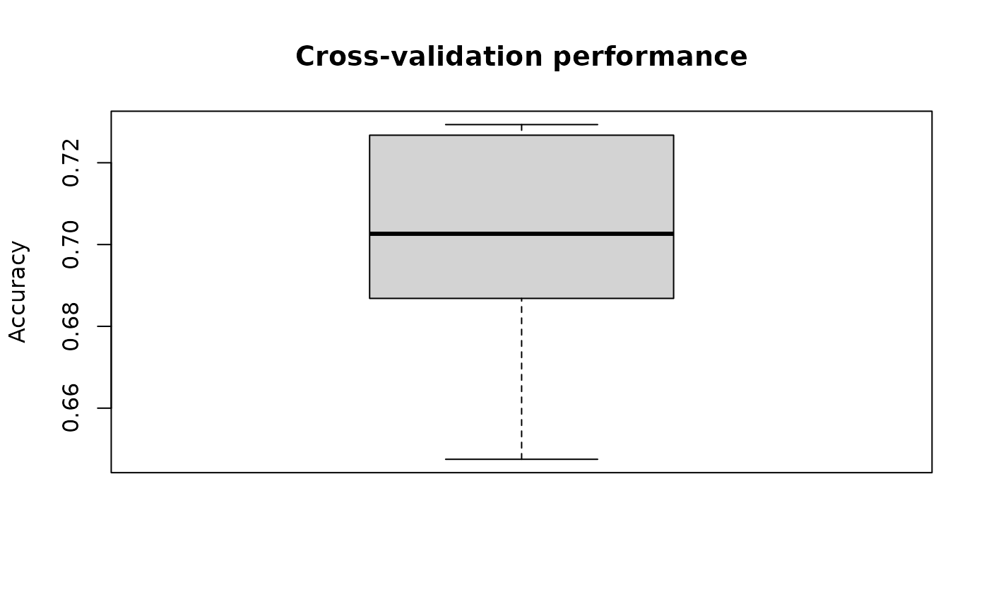
Fig.1 Mean cross-validation accuracy across repeats.
Without Cross-validation
In this example, we show a simpler case without cross validation, where we have a prediction that we want to compare with the ground truth directly. For example, we may have simulated a single-cell count matrix and want to compare with an experimental count matrix on various attributes.
Here, we use the microbiome dataset to demonstrate the above case.
Step 1: Simulate a matrix of the same size as the microbiome data using negative binomial. Step 2: Define a function that calculate the sparsity of a given matrix. Step 3: Define a metric that compare difference of two values. Step 4: Evaluate the difference in sparsity of the microbiome data and the simulated data.
set.seed(1)

# generate a simulated matrix
sim <- rnbinom(nrow(x) * ncol(x), size = 1, mu = 1)
sim <- Matrix(sim, nrow = nrow(x), ncol = ncol(x))

# function that calculate the sparsity of a matrix
calc_sparsity <- function(data) {
  sparsity <- sum(data == 0) / length(data)
  return(sparsity)
}


# metric that compare the difference of two values
calc_diff <- function(evidence, predicted) {
  return(predicted - evidence)
}
# add metric that we just defined
trio$addMetric(name = "Difference", metric = calc_diff)

# calculate the sparsity of the data, and then input into the supporting evidence
trio$addEvidence(name = "Sparsity", evidence = calc_sparsity, metrics = "Difference")

# because we used negative binomial to simulate a matrix
# we will name the method as "negative binomial"
# then calculate the sparsity of the simulated matrix
# and compare with the Sparsity supporting evidence
eval_res <- trio$evaluate(
  list(negative_binomial = list(Sparsity = sim))
)

eval_res
## # A tibble: 1 × 5
## datasetID method evidence metric result
## <chr> <chr> <chr> <chr> <dbl>
## 1 lubomski_microbiome negative_binomial Sparsity Difference -0.323From the evaluation result, we see there is a -0.32 difference in the sparsity between the microbiome data and the data simulated with negative binomial.
Importing result to BenchmarkInsights
The result dataframe obtained from Trio evaluation can
be passed to BenchmarkInsights for subsequent
visualisation. BenchmarkInsights is another structure in
BenchHub that provide a list of functions to analyse and
visualise the benchmarking results from multiple perspectives.
Note, to make the result dataframe compatible for BenchmarkInsights, please make sure the dataframe is in the format shown below, where the column names are “datasetID”, “method”, “evidence”, “metric” , “result”, and that there is one row for each result.
# in the with cross validation result, we need to average the results from multiple repeats to give one value
result <- result %>%
  dplyr::group_by(datasetID, method, evidence, metric) %>%
  dplyr::summarize(result = mean(result))
## `summarise()` has regrouped the output.
## ℹ Summaries were computed grouped by datasetID, method, evidence, and metric.
## ℹ Output is grouped by datasetID, method, and evidence.
## ℹ Use `summarise(.groups = "drop_last")` to silence this message.
## ℹ Use `summarise(.by = c(datasetID, method, evidence, metric))` for
## per-operation grouping (`?dplyr::dplyr_by`) instead.
result <- rbind(result, eval_res)
result
## # A tibble: 2 × 5
## # Groups: datasetID, method, evidence [2]
## datasetID method evidence metric result
## <chr> <chr> <chr> <chr> <dbl>
## 1 lubomski_microbiome lasso Diagnosis Balanced Accuracy 0.699
## 2 lubomski_microbiome negative_binomial Sparsity Difference -0.323Please see Vignette 3 for the details on the visualisations and
functions in BenchmarkInsights.
Session Info
## R version 4.6.0 (2026-04-24)
## Platform: x86_64-pc-linux-gnu
## Running under: Ubuntu 24.04.4 LTS
##
## Matrix products: default
## BLAS:   /usr/lib/x86_64-linux-gnu/openblas-pthread/libblas.so.3
## LAPACK: /usr/lib/x86_64-linux-gnu/openblas-pthread/libopenblasp-r0.3.26.so;  LAPACK version 3.12.0
##
## locale:
##  [1] LC_CTYPE=C.UTF-8       LC_NUMERIC=C           LC_TIME=C.UTF-8
##  [4] LC_COLLATE=C.UTF-8     LC_MONETARY=C.UTF-8    LC_MESSAGES=C.UTF-8
##  [7] LC_PAPER=C.UTF-8       LC_NAME=C              LC_ADDRESS=C
## [10] LC_TELEPHONE=C         LC_MEASUREMENT=C.UTF-8 LC_IDENTIFICATION=C
##
## time zone: UTC
## tzcode source: system (glibc)
##
## attached base packages:
## [1] stats     graphics  grDevices utils     datasets  methods   base
##
## other attached packages:
##  [1] glmnet_4.1-10    Matrix_1.7-5     lubridate_1.9.5  forcats_1.0.1
##  [5] stringr_1.6.0    dplyr_1.2.1      purrr_1.2.2      readr_2.2.0
##  [9] tidyr_1.3.2      tibble_3.3.1     ggplot2_4.0.3    tidyverse_2.0.0
## [13] BenchHub_0.99.15 BiocStyle_2.39.0
##
## loaded via a namespace (and not attached):
##  [1] gridExtra_2.3          httr2_1.2.2            rlang_1.2.0
##  [4] magrittr_2.0.5         compiler_4.6.0         survAUC_1.4-0
##  [7] systemfonts_1.3.2      vctrs_0.7.3            reshape2_1.4.5
## [10] shape_1.4.6.1          pkgconfig_2.0.3        fastmap_1.2.0
## [13] backports_1.5.1        utf8_1.2.6             ggstance_0.3.7
## [16] rmarkdown_2.31         tzdb_0.5.0             ragg_1.5.2
## [19] xfun_0.57              cachem_1.1.0           jsonlite_2.0.0
## [22] broom_1.0.12           cluster_2.1.8.2        R6_2.6.1
## [25] bslib_0.10.0           stringi_1.8.7          RColorBrewer_1.1-3
## [28] rpart_4.1.27           jquerylib_0.1.4        cellranger_1.1.0
## [31] Rcpp_1.1.1-1.1         bookdown_0.46          iterators_1.0.14
## [34] knitr_1.51             base64enc_0.1-6        parameters_0.28.3
## [37] splines_4.6.0          nnet_7.3-20            timechange_0.4.0
## [40] tidyselect_1.2.1       rstudioapi_0.18.0      yaml_2.3.12
## [43] codetools_0.2-20       curl_7.1.0             lattice_0.22-9
## [46] plyr_1.8.9             withr_3.0.2            bayestestR_0.17.0
## [49] S7_0.2.2               evaluate_1.0.5         marginaleffects_0.32.0
## [52] foreign_0.8-91         desc_1.4.3             survival_3.8-6
## [55] pillar_1.11.1          BiocManager_1.30.27    checkmate_2.3.4
## [58] foreach_1.5.2          insight_1.5.0          generics_0.1.4
## [61] hms_1.1.4              scales_1.4.0           glue_1.8.1
## [64] Hmisc_5.2-5            tools_4.6.0            data.table_1.18.2.1
## [67] fs_2.1.0               grid_4.6.0             datawizard_1.3.1
## [70] colorspace_2.1-2       googlesheets4_1.1.2    patchwork_1.3.2
## [73] performance_0.16.0     htmlTable_2.5.0        googledrive_2.1.2
## [76] splitTools_1.0.1       Formula_1.2-5          cli_3.6.6
## [79] rappdirs_0.3.4         textshaping_1.0.5      gargle_1.6.1
## [82] gtable_0.3.6           ggcorrplot_0.1.4.1     ggsci_5.0.0
## [85] sass_0.4.10            digest_0.6.39          ggrepel_0.9.8
## [88] htmlwidgets_1.6.4      farver_2.1.2           htmltools_0.5.9
## [91] pkgdown_2.2.0          lifecycle_1.0.5        dotwhisker_0.8.4