Downstream analysis
Sydney Precision Bioinformatics Group
18 June 2019
1 Introduction
We have now preprocessed and merged our single cell data. The next step is to analyse the data for cell type identification, identification of marker genes and et cetera. We will focus on some simple steps of downstream analysis for single cell RNA-sequencing (scRNA-seq) data as shown below.
- What are the cell types present in the dataset?
- What are these cell clusters?
- For a gene of interest, how can I visualise the gene expression distribution?
- What are the cell type composition in the data?
We will be using some of the functions we developed in our scdney package. You may visit our package website for the vignette and further details about scdney.
1.1 Loading packages
suppressPackageStartupMessages({
  library(SingleCellExperiment)
  library(SummarizedExperiment)
  library(dplyr)
  library(edgeR)
  library(scdney)
  library(mclust)
  library(Rtsne)
  library(parallel)
  library(cluster)
  library(ggplot2)
  library(MAST)
  library(viridis)
  library(ggpubr)
  library(plyr)
  library(monocle)
})

theme_set(theme_classic(16))
1.2 Loading data
In the scMerge publication, we have merged four mouse liver datasets together. This data is a bit too large for us to work with in this workshop, hence, we will take the merged data with all four datasets and subset ourselves to only the Su and Yang datasets. Some processings were performed in this data compare to the previous section, namely, the Megakaryocyte, Erythrocyte cells from the previous section are labelled as Hematopoietic cells in this section.
datapath = "./data/"
# datapath = "/home/data/"
sce_scMerge = readRDS(paste0(datapath, "liver_scMerge.rds"))

## We will subset Su et al. and Yang et al. datasets.
ids = colData(sce_scMerge)$batch %in% c("GSE87795", "GSE90047")

subset_data = sce_scMerge[,ids]

lab = colData(subset_data)$cellTypes

nCs = length(table(lab))

mat = SummarizedExperiment::assay(subset_data, "scMerge")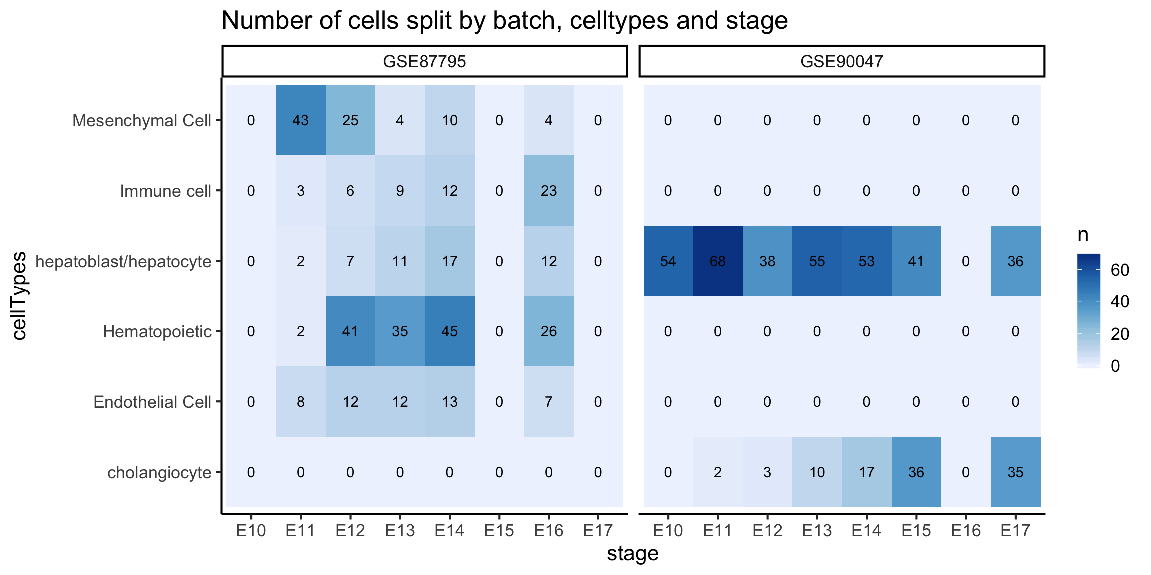
2 Q1. What are the cell types present in the dataset?
Typically, a single cell RNA-sequencing experiment does not come with labelled cell type information for individual cells. We will need to identify cell types of indivdual cells in our data with bioinformatics analysis.
Before we identify the cell types in the dataset, we need to first identify how many distinct group of population we can find from our data. One common method to achieve this is a statistical technique called clustering. A clustering method will group similar samples (cells) together and partition samples that are different by comparing their feature information (gene expression).
There are two components that ultimately determine the performance of a clustering method:
- The similarity metric that determines if two cells are similar to each other, and
- The algorithm itself that uses the similarity metric to perform the grouping operations.
In our recent study, we found Pearson correlation to be the optimal similarity metric for comparing single cell RNA-seq data ( Kim et al., 2018 ). Therefore in this workshop, we will utilise scClust in our scdney package, which implemented 2017 Nature methods clustering algorithm SIMLR with pearson correlation.
2.1 How many distinct group of population are there in my dataset?
Typical clustering methods (except for some methods like hierarchical clustering) require users to specify number of distinct groups (k) to cluster from your data. In the context of this data, we can think of k as the the number of cell types.
In an unsupervised setting, we do not know the exact number and therefore, in a practical setting, we should run clustering for various number of k and evaluate their clustering performance.
However, due to the time limit of this workshop, we will only run the scClust clustering for k = 6 as a demonstration and load a saved result with more values of k computed.
## For demonstration purpose, we will run k = 6 (which is actually the number of cell types in our dataset)
simlr_result_k6 = scClust(mat, 6, similarity = "pearson", method = "simlr", seed = 1, cores.ratio = 0, geneFilter = 0)

load("data/simlr.results.RData")
[Extension] If you are interested, this is how you can compute data/simlr.results.RData by yourself.
## We will NOT run for various `k` to save time. Instead, we will load pre-computed results for `k` between 3 to 8

## This is an easy way to run `scClust` for k = 3, 4, 5, 6, 7, 8.
all_k = 3:8
simlr_results = sapply(as.character(all_k), function(k) {
  scClust(mat, as.numeric(k), similarity = "pearson", method = "simlr", seed = 1, cores.ratio = 0, geneFilter = 0)
}, USE.NAMES = TRUE, simplify = FALSE)
2.2 How do we select optimal k?
If our k is optimal, we should expect that the each cluster are closely packed together and the distances within the clusters, within-cluster sum of squares (WSS) are expected to be small. Thus, we will select the k with a small total WSS (compact clusters). This is called the “elbow” method.
# Find total WSS from all cluster outputs
all_wss = sapply(simlr_results, function(result) {
  sum(result$y$withinss)
}, USE.NAMES = TRUE, simplify = TRUE)

plot_data = data.frame(
  k = as.integer(names(all_wss)),
  total_wss = all_wss
)

ggplot(plot_data,
       aes(x = k,
           y = total_wss)) +
  geom_point(size = 3) +
  stat_smooth(method = loess, col = "red",
              method.args = list(degree = 1), se = FALSE) +
  labs(title = "Compare Total WSS for each k",
       y = "Total WSS")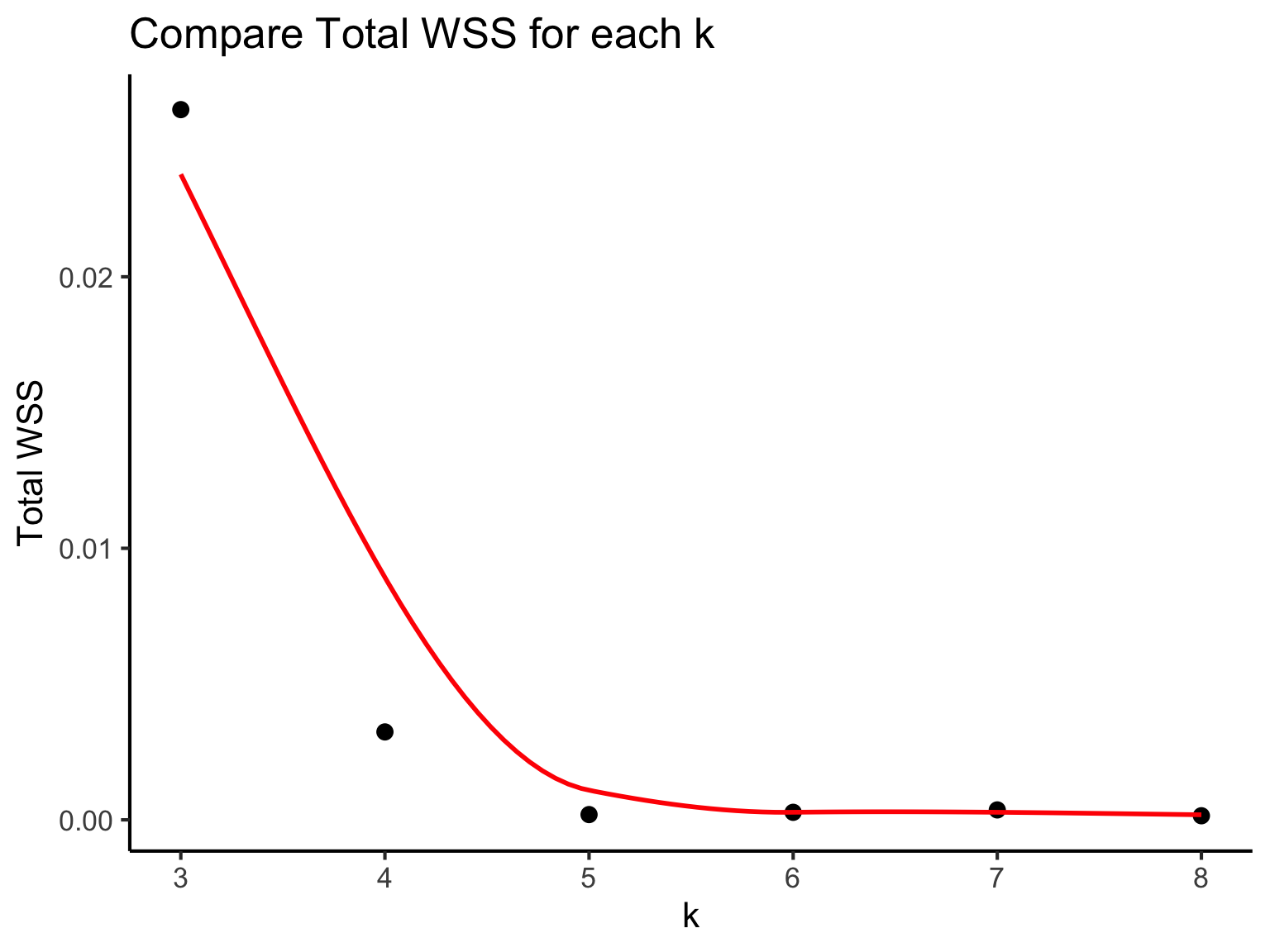
As shown in this plot, the graph begin to plateau from k = 5. We can estimate that k is around 5 or 6. We can further investigate using silhouette scores or other metrics but using our t-SNE plot (this may require a bit of practical experience) we will estimate k = 6.
Quick quiz
- We can determine
kwith compactness of the clusters. What other measure can we use to determinek? - How would you determine optimal number of clusters for hierarchical clustering?
2.3 Effect of similarity metrics
For the purpose of demonstration, we would like to highlight the effect of similarity metric to your cluster output. We will first compute a t-SNE plot and then overlay that with
- Clustering result using Pearson correlation
- Clustering result using Euclidean distance
- True cell type labels from the publications
## To run scClust with euclidean distance, uncommnet the following lines.
## simlr_result_eucl_k6 = scClust(mat, 6, similarity = "euclidean", method = "simlr", seed = 1, cores.ratio = 0, geneFilter = 0)

## for convenience, we will load our pre-computed result
load(paste0(datapath, "simlr_result_eucl_k6.RData"))
# create tsne object
set.seed(123)
tsne_result = Rtsne(t(mat), check_duplicates = FALSE)
#################################################
tmp_lab = as.numeric(factor(lab))
pear_cluster = plyr::mapvalues(
simlr_result_k6$y$cluster,
from = c(1,2,3,4,5,6),
to = c(2,3,1,4,6,5)
)
eucl_cluster = plyr::mapvalues(
simlr_result_eucl_k6$y$cluster,
from = c(1,2,3,4,5,6),
to = c(6,2,4,3,1,5)
)
#################################################
plot_data = data.frame(
tsne1 = rep(tsne_result$Y[,1], 3),
tsne2 = rep(tsne_result$Y[,2], 3),
cluster = factor(c(tmp_lab, pear_cluster, eucl_cluster)),
label = rep(c("Truth", "Pearson", "Euclidean"), each = length(lab)))
ggplot(plot_data, aes(x = tsne1, y = tsne2, colour = cluster)) +
geom_point(size = 2) +
labs(title = "t-SNE plot") +
facet_grid(~label) +
theme(legend.position = "none")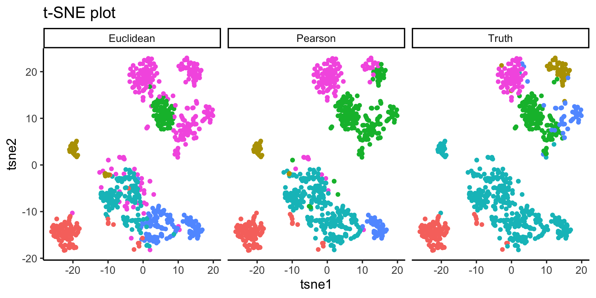
plot_data2 = data.frame(
  Truth = lab,
  computed_cluster = as.factor(c(pear_cluster, eucl_cluster)),
  label = rep(c("Pearson", "Euclidean"), each = length(lab))
)


plot_data2 %>%
  dplyr::group_by(Truth, computed_cluster, label) %>%
  dplyr::summarise(n = n()) %>%
  dplyr::ungroup() %>%
  tidyr::complete(Truth, computed_cluster, label, fill = list(n = 0)) %>%
  ggplot(aes(x = computed_cluster,
             y = Truth,
             fill = n, label = n)) +
  geom_tile() +
  geom_text() +
  facet_wrap(~label) +
  scale_fill_distiller(palette = "Blues", direction = 1) +
  labs(title = "")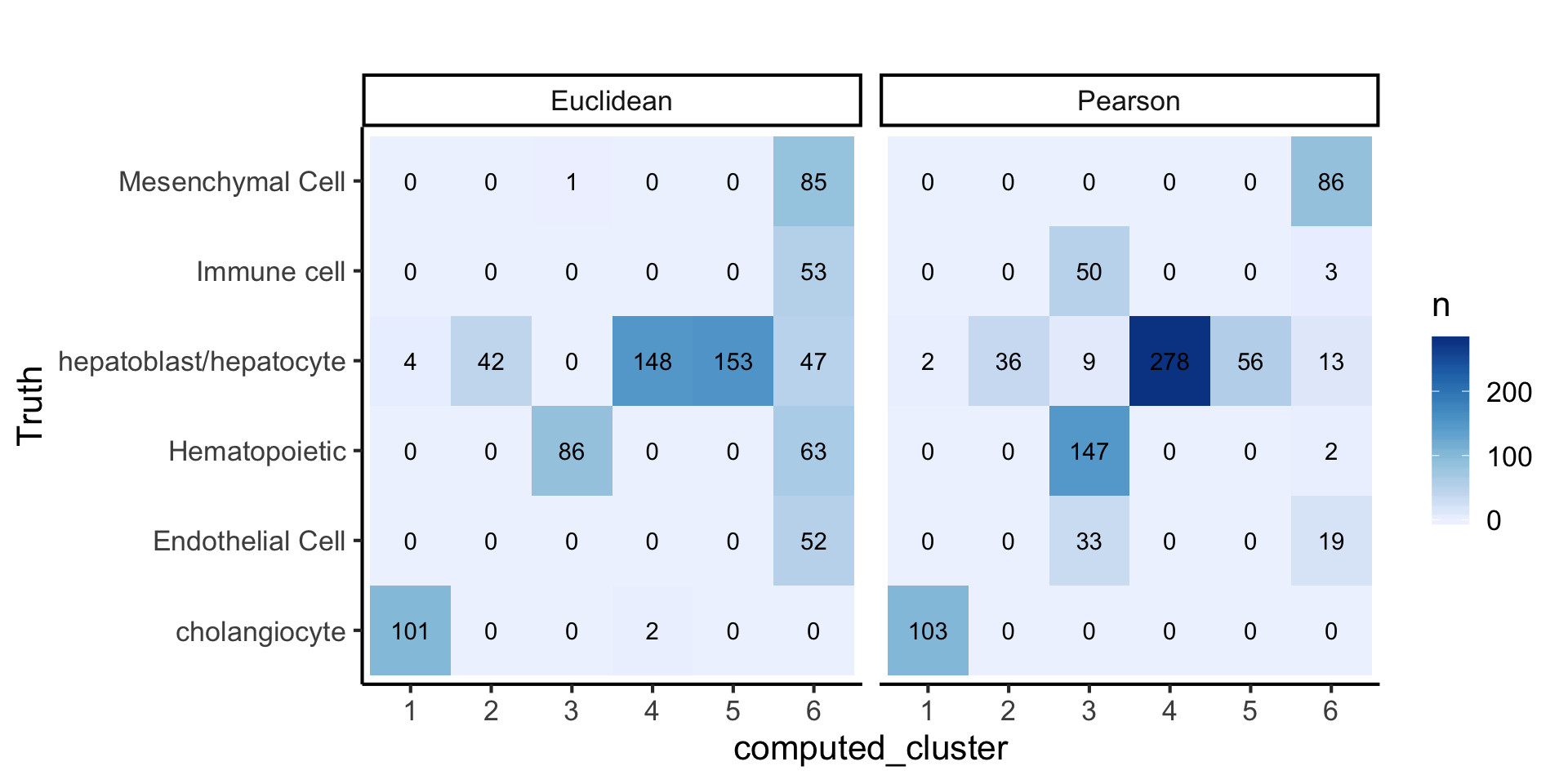
Quick quiz
- From your observation of the above t-SNE plot, did our clustering method (with Pearson correlation) group cells well?
[Optional] We can evaluate the clustering performance using the cell type labels providede from the publications.
# ARI
ari = c(mclust::adjustedRandIndex(lab, simlr_result_eucl_k6$y$cluster),
        mclust::adjustedRandIndex(lab, simlr_result_k6$y$cluster))

# NMI
nmi = c(igraph::compare(as.numeric(factor(lab)),
                        simlr_result_eucl_k6$y$cluster, method = "nmi"),
        igraph::compare(as.numeric(factor(lab)),
                        simlr_result_k6$y$cluster, method = "nmi"))

plot_data = data.frame(
  dist = rep(c("Euclidean", "Pearson"), 2),
  value = c(ari, nmi),
  eval = rep(c("ARI", "NMI"), each = 2)
)

ggplot(plot_data, aes(x = dist, y = value, fill = dist)) +
  geom_bar(stat="identity") +
  facet_grid(col = vars(eval)) +
  labs(x = "Similarity metrics",
       y = "Evalution score",
       title = "Affect of similarity metrics in scRNA-seq data") +
  theme(legend.position = "none")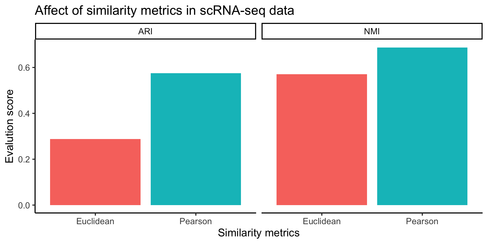
3 Q2. What are these cell clusters?
Now that we have clustered all the cells to 6 distinct groups, we may want to find out what these clusters are, i.e. what cell types are there in my dataset? Thus, we may ask what defines a cell type?
We can use marker genes to identify cell types.
3.1 2.1 What are the marker genes that distinguish the different cell types?
Here we provide a function that allow one to find differentially expressed gene between a cluster and the remaining clusters. The input of this function is the expression matrix and the cluster ID. The output is a list of marker genes and their associated p-values.
Here we provide an example of using the findmarker function.
To find out the marker genes in cluster 4, we type in 4 in the findmarker function. We then look at the top 10 genes ranked by p-value. We can then use ggplot to visualise the distribution of one of the genes across the dataset.
marker_cluster4 = findMarker(mat = mat,
                             cluster = simlr_result_k6$y$cluster,
                             cluster_id = 4)
marker_cluster4[1:10, ]## gene P_value
## 12739 Gys2 6.068095e-153
## 19151 Shbg 2.513240e-134
## 12924 Hgd 1.577501e-126
## 19364 Slc27a2 8.229521e-124
## 6096 Gcgr 7.663681e-122
## 16209 Otc 1.338106e-115
## 12842 Hc 1.016114e-113
## 15057 Mogat2 1.509759e-113
## 12729 Gulo 6.801648e-113
## 14081 Lect2 1.976735e-112tsne_plotdf = data.frame(
tsne1 = tsne_result$Y[, 1],
tsne2 = tsne_result$Y[, 2]) %>%
dplyr::mutate(
cluster = as.factor(simlr_result_k6$y$cluster),
Gys2 = mat["Gys2", ])
ggplot(data = tsne_plotdf, aes(x = tsne1, y = tsne2, colour = Gys2) ) +
geom_point(alpha = 0.5) +
scale_color_viridis() +
labs(col = "Gys2 expression", x = "tsne1", y = "tsne2")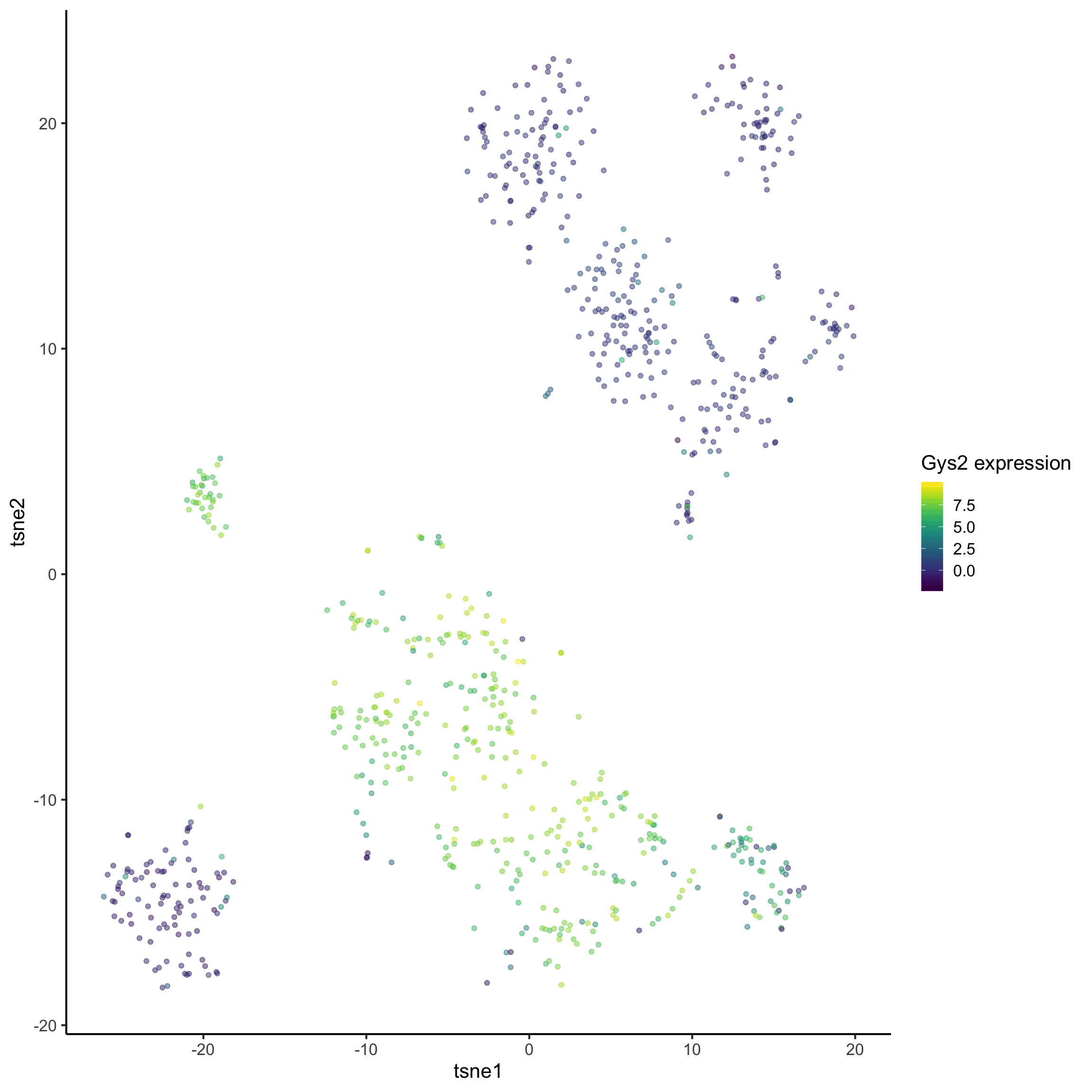
Quick quiz
What does the above t-SNE plot tell you?
Here we repeat the analysis as above, but for cluster 3. See if you can understand the output.
marker_cluster3 = readRDS(paste0(datapath, "marker_cluster3.rds"))tsne_plotdf = tsne_plotdf %>%
dplyr::mutate(Erich5 = mat["Erich5",])
ggplot(data = tsne_plotdf,
mapping = aes(x = tsne1, y = tsne2, colour = Erich5)) +
geom_point(alpha = 0.5) +
scale_color_viridis() +
labs(col="Erich5 expression")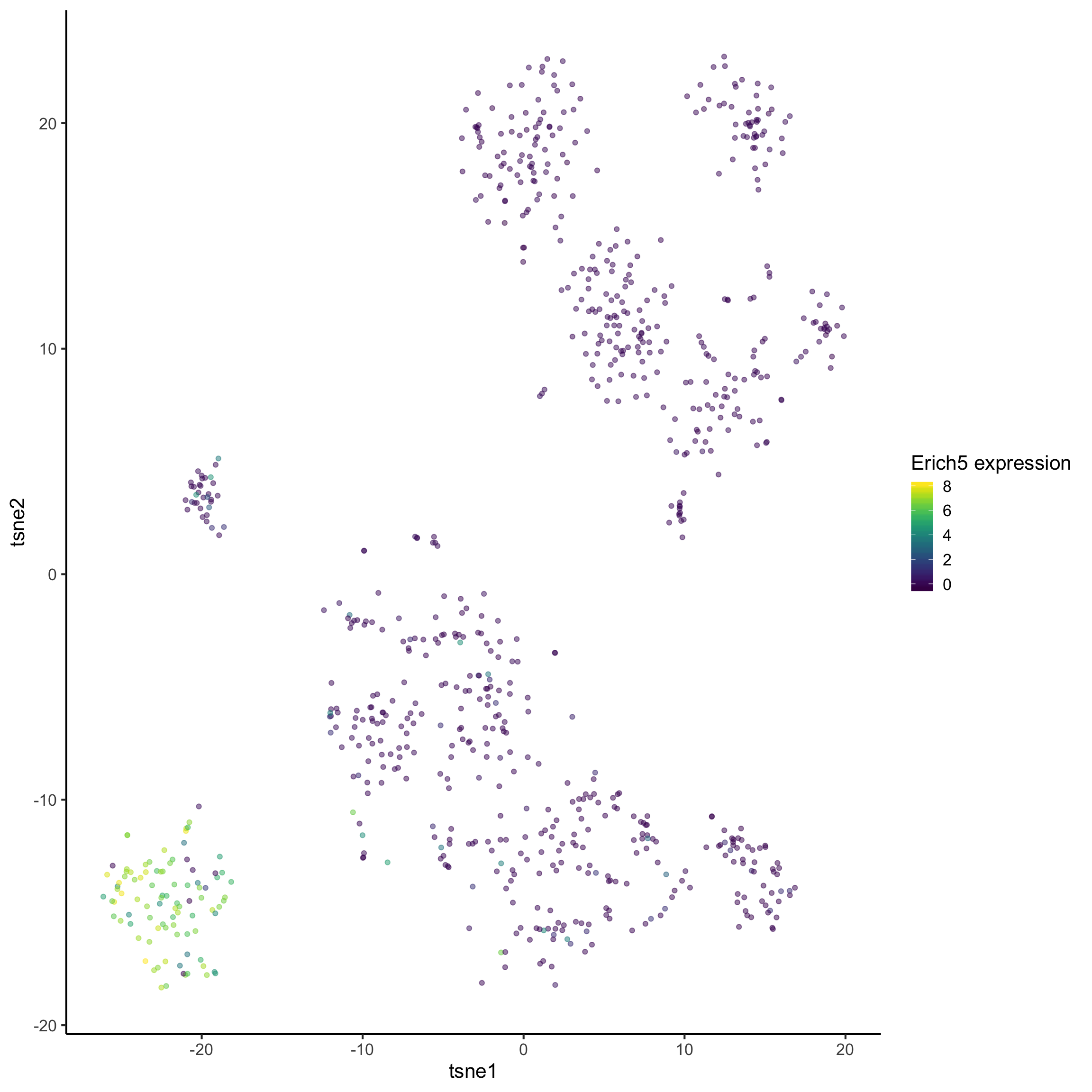
4 Q3. For a gene of interest, how can I visualise the gene expression distribution?
In Q2, we have identified some interesting marker genes from our dataset. If we have a gene that we know, and we want to identify the its expression pattern in our dataset, we can also visualise the distribution. For example, Hnf4a has been stated in literature as a marker gene for hepatoblast cell (citation).
The figure on the left highlight cluster 4 and the figure on the right highlight the expression of Hnf4a.
This suggests that cluster 4 could belong to hepatoblast cell.
tsne_plotdf = tsne_plotdf %>%
  dplyr::mutate(Hnf4a = mat["Hnf4a",])


fig1 = ggplot(data = tsne_plotdf,
              mapping = aes(x = tsne1, y = tsne2)) +
  geom_point(aes(color = ifelse(cluster == 4, 'Yellow', 'Purple')), alpha = 0.5) +
  scale_colour_viridis_d() +
  labs(x = "",
       y = "",
       title = "Cluster 4") +
  theme(legend.position = "none")


fig2 = ggplot(data = tsne_plotdf,
              mapping = aes(x = tsne1, y = tsne2, colour = Hnf4a) ) +
  geom_point(alpha = 0.5) +
  scale_color_viridis() +
  labs(x = "",
       y = "",
       title = "Hnf4a expression pattern")

ggarrange(fig1,fig2, ncol= 2, nrow = 1)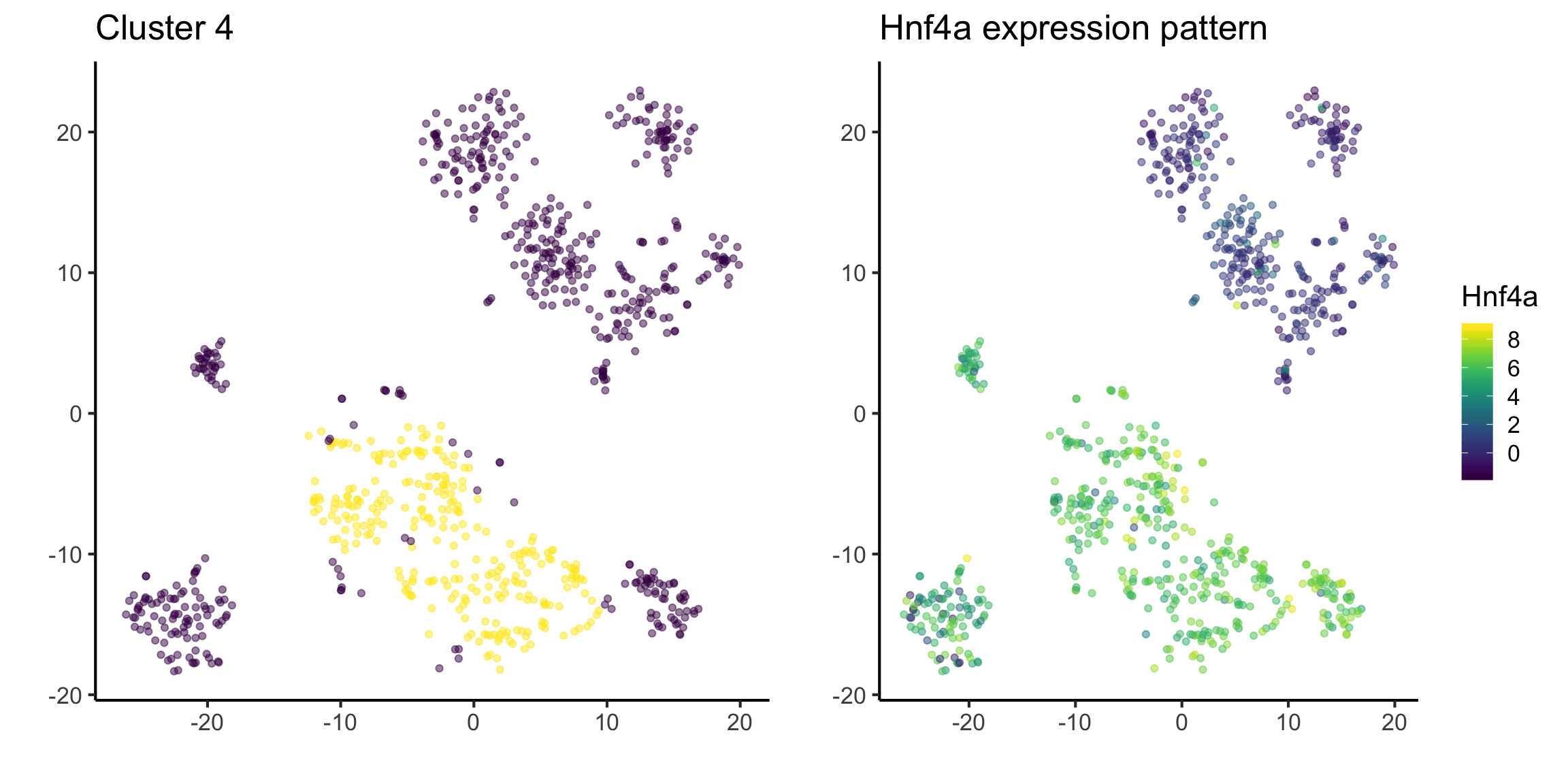
Quick quiz
See if you can understand the output of the following code.
tsne_plotdf = tsne_plotdf %>%
  dplyr::mutate(Epcam = mat["Epcam",])


fig1 = ggplot(data = tsne_plotdf, mapping = aes(x = tsne1, y = tsne2) ) +
  geom_point(aes(color = ifelse(cluster == 3, 'Yellow', 'Purple')), alpha = 0.5) +
  scale_colour_viridis_d() +
  labs(x = "",
       y = "",
       title = "Cluster 3") +
  theme(legend.position = "none")


fig2 = ggplot(data = tsne_plotdf,
               mapping = aes(x = tsne1, y = tsne2, colour = Epcam) ) +
  geom_point(alpha=0.5) +
  scale_color_viridis() +
  labs(x = "",
       y = "",
       title = "Epcam expression pattern")

ggarrange(fig1,fig2, ncol= 2, nrow = 1)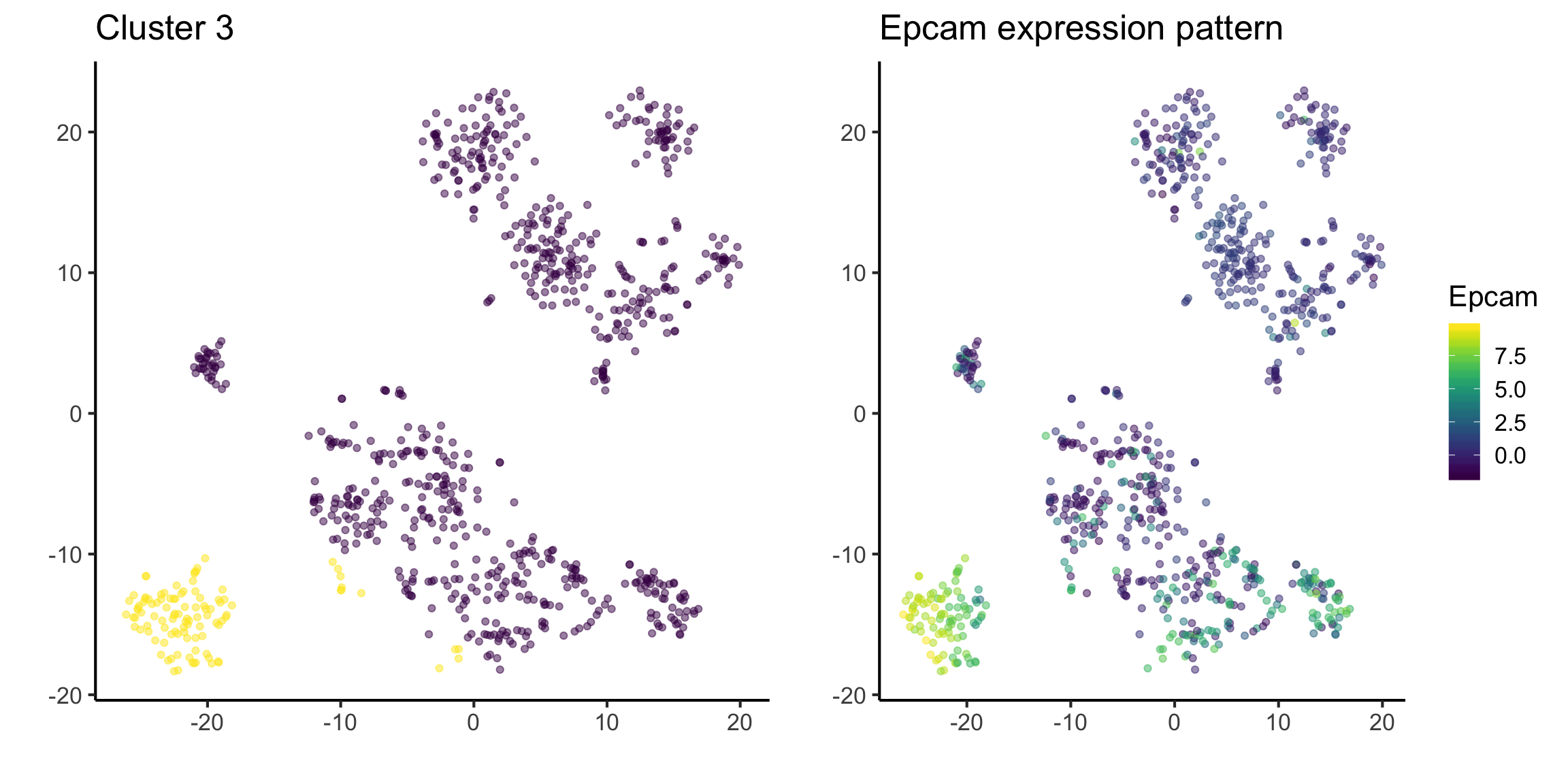
As you may have already noticed from above steps, unsupervised clustering methods alone are not perfect in capturing cell type information. Using this step iteratively, we need to refine our cell type information.
5 Q4. What are the cell type composition in the data?
NOTE: From this step, we will assume we have correctly refined our cell type information from above steps and we will use the cell type information provided in Su et. al. 2017 and Yang et. al. 2017.
5.1 Cell type proportions
plot_data = data.frame(table(lab)) %>%
  dplyr::mutate(lab = reorder(lab, Freq))

ggplot(plot_data,
       aes(x = lab,
           y = Freq,
           fill = lab)) +
  geom_bar(stat = "identity") +
  labs(x = "Cell types",
       y = "Frequency",
       title = "Composition of cell types") +
  theme(legend.position = "none")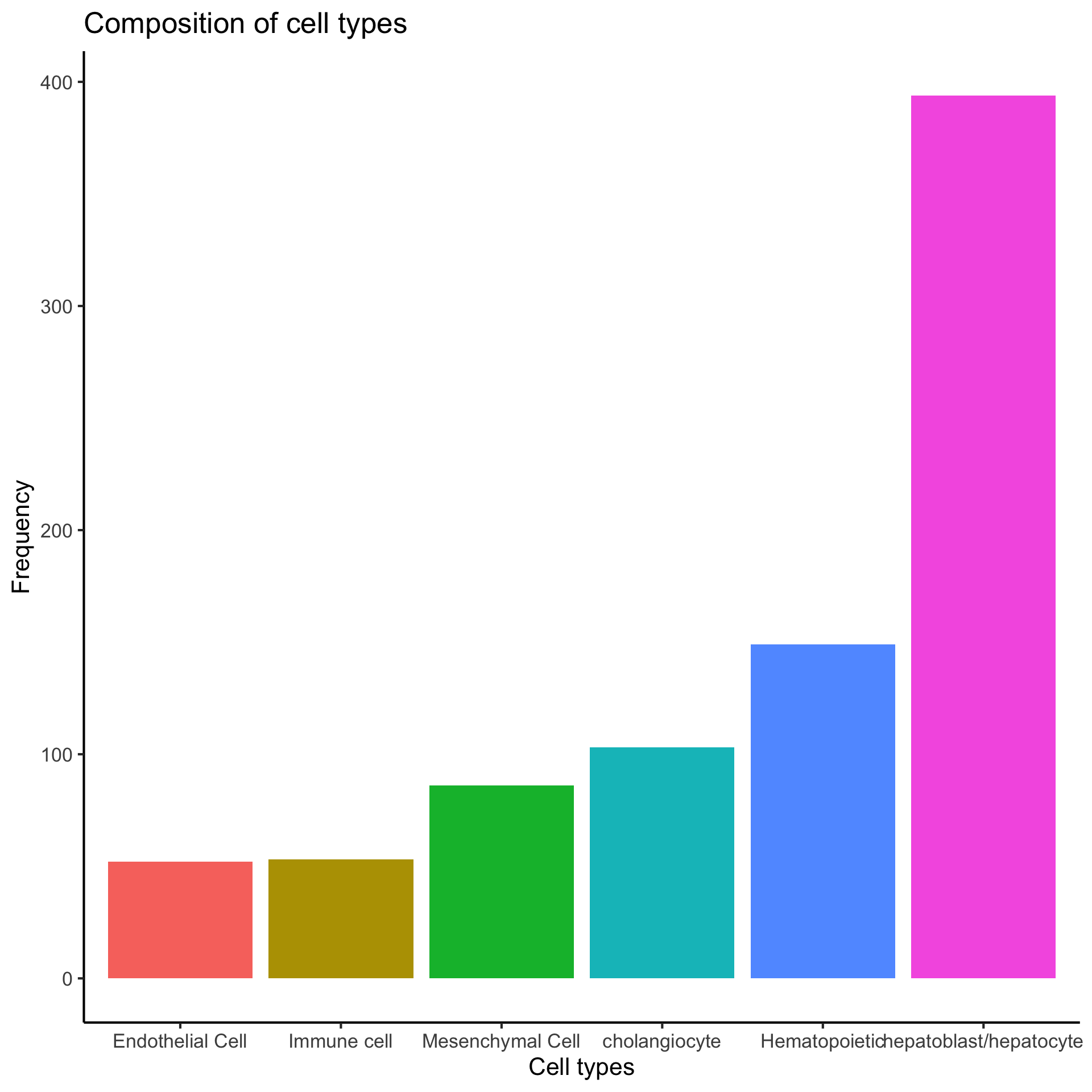
We observe that hepatoblast/hepatocyte is the largest population.
6 Extension: Any rare cell type? What is the most common cell type?
7 Extension: Monocle
A popular question in scRNA-Seq analysis is if the gene expressions patterns changes over some time.
The monocle method is a well-established psuedo-time trajectory reconstruction method from Trapnell et. al. (2014). You can learn more about the theoretical construction of monocle here. In terms of computations, monocle requires some psuedo-time modelling on each gene and then markers are selected to perform psuedo-time ordering.
The code below construct psuedo-time trajectory for the Hepatoblast/Hepatocyte cells in the merged data.
## Subsetting data to "hepatoblast/hepatocyte"
monocle_data = subset_data[,colData(subset_data)$cellTypes %in% c("hepatoblast/hepatocyte")]
## Add a "stage" column to the colData of the monocle_data
colData(monocle_data)$stage = stringr::str_sub(colnames(monocle_data), 1, 3)
table(colData(monocle_data)$stage)
##
## E10 E11 E12 E13 E14 E15 E16 E17
## 54 70 45 66 70 41 12 36## monocle needs a rowData (data about each gene)
rowData(monocle_data) = DataFrame(gene_short_name = rownames(monocle_data))
monocle_data## class: SingleCellExperiment
## dim: 22864 394
## metadata(0):
## assays(1): scMerge
## rownames(22864): Gm19938 Sox17 ... Gm47123 Gm48236
## rowData names(1): gene_short_name
## colnames(394): E11.5_C06 E11.5_C12 ... E17.5D_4_05 E17.5E_4_10
## colData names(3): cellTypes batch stage
## reducedDimNames(0):
## spikeNames(0):
## altExpNames(0):## moncole requires a `CellDataSet` object to run.
## You can convert monocle_data into a `CellDataSet` object using the scran package.
monocle_CellDataSet = scran::convertTo(
monocle_data,
type = "monocle",
assay.type = "scMerge"
# col.fields = c("cellTypes", "stage", "batch"),
# row.fields = c("gene_short_name")
) %>%
estimateSizeFactors()
## Performing differential gene test using "stage".
diff_test_res = differentialGeneTest(
monocle_CellDataSet, fullModelFormulaStr = "~stage")
## We will select the top genes to be used for clustering and
## calculate dispersion (variability) parameters before constructing the trajectory
ordering_genes = row.names(subset(diff_test_res, qval < 0.00001))
length(ordering_genes)## [1] 868monocle_CellDataSet = setOrderingFilter(monocle_CellDataSet, ordering_genes)
monocle_CellDataSet = estimateDispersions(monocle_CellDataSet) %>% suppressWarnings()
# plot_ordering_genes(monocle_CellDataSet)
## Construcing the trajectory
monocle_CellDataSet = reduceDimension(monocle_CellDataSet,
max_components = 2,
method = 'DDRTree')
monocle_CellDataSet = orderCells(monocle_CellDataSet)
plot_cell_trajectory(monocle_CellDataSet, color_by = "stage")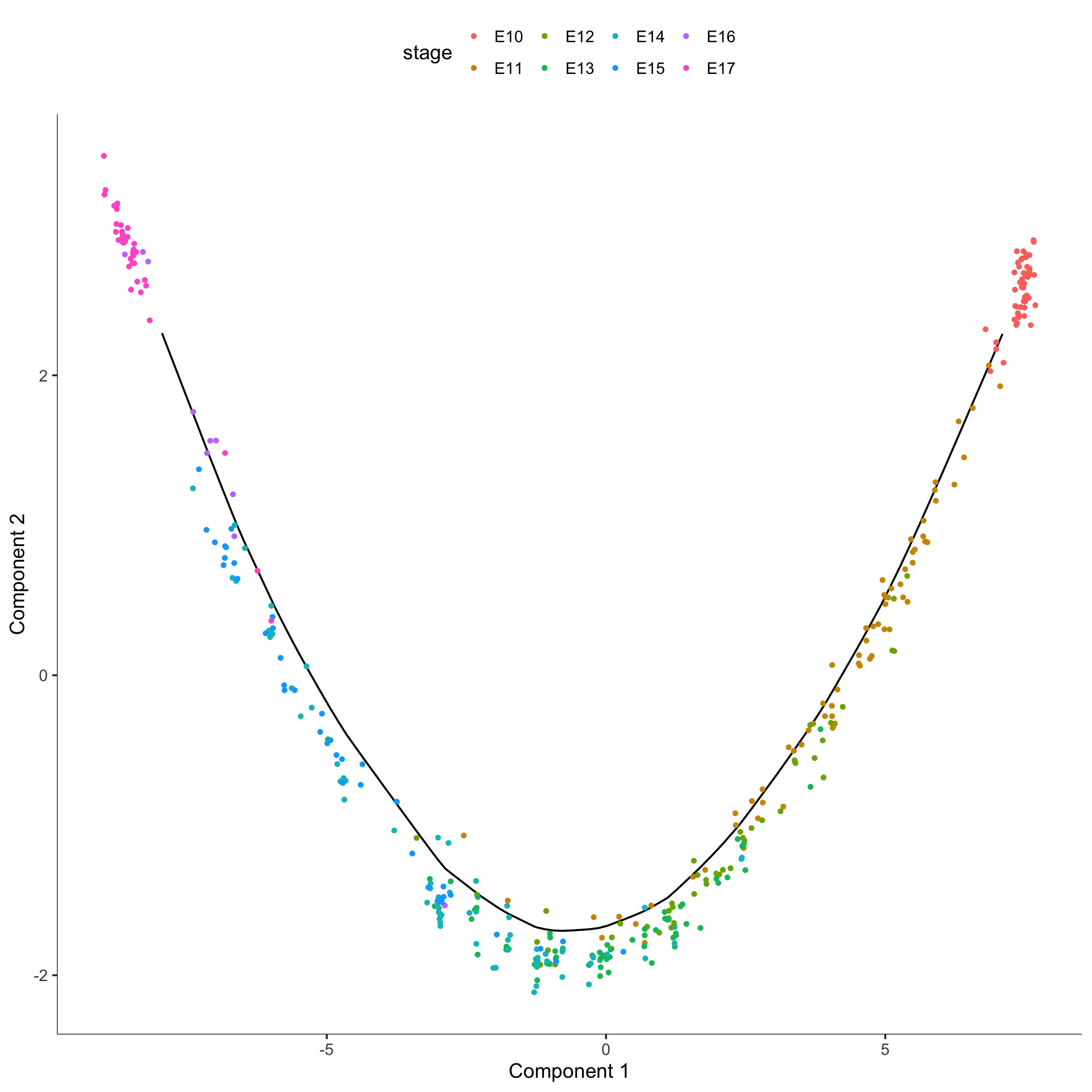
# monocle::plot_cell_clusters(monocle_CellDataSet)
plot_genes_in_pseudotime(monocle_CellDataSet[c("Sarm1", "Gm38388"),], color_by = "stage")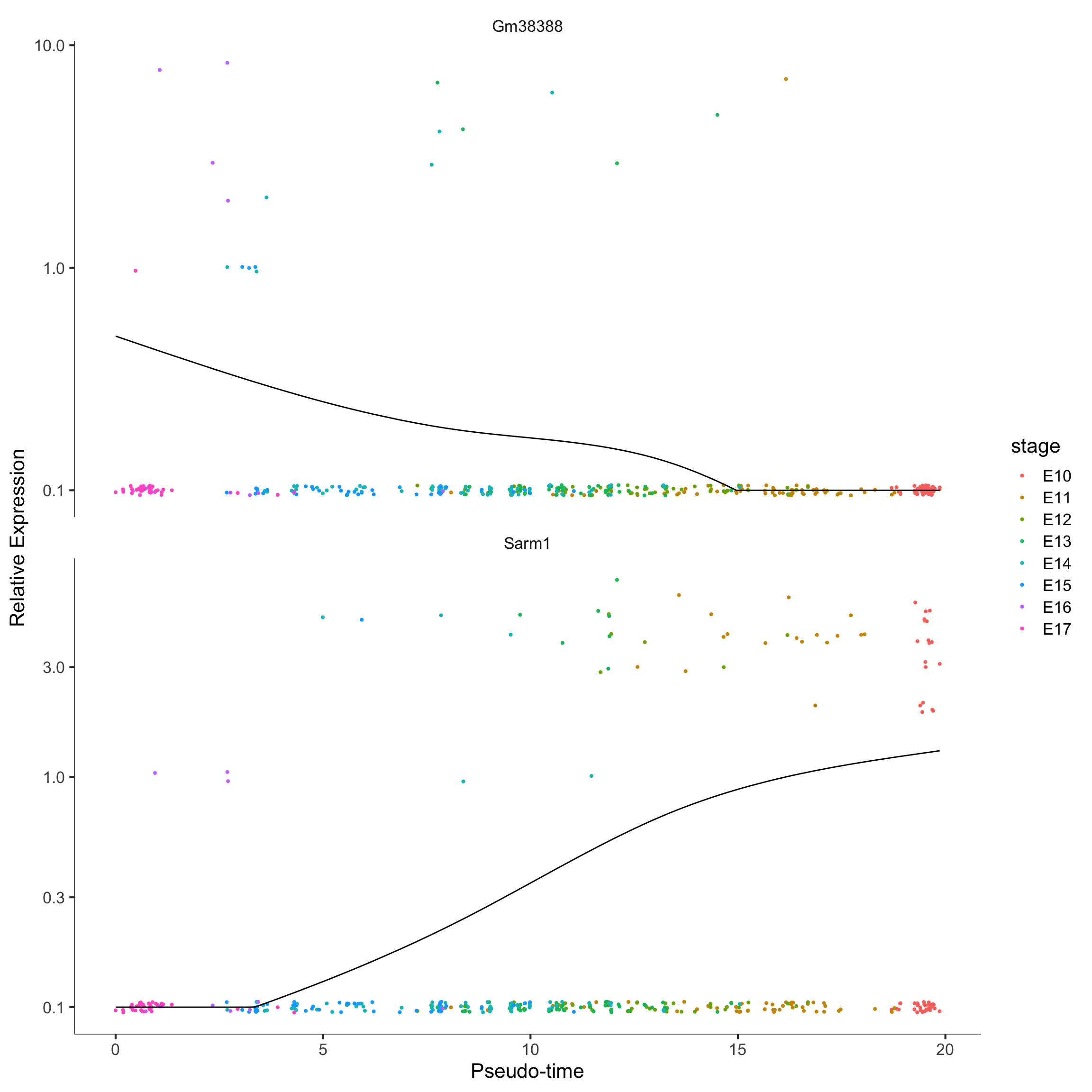
8 SessionInfo
sessionInfo()## R version 3.6.0 (2019-04-26)
## Platform: x86_64-apple-darwin15.6.0 (64-bit)
## Running under: macOS High Sierra 10.13.6
##
## Matrix products: default
## BLAS: /Library/Frameworks/R.framework/Versions/3.6/Resources/lib/libRblas.0.dylib
## LAPACK: /Library/Frameworks/R.framework/Versions/3.6/Resources/lib/libRlapack.dylib
##
## locale:
## [1] en_AU.UTF-8/en_AU.UTF-8/en_AU.UTF-8/C/en_AU.UTF-8/en_AU.UTF-8
##
## attached base packages:
## [1] splines parallel stats4 stats graphics grDevices utils
## [8] datasets methods base
##
## other attached packages:
## [1] monocle_2.13.0 DDRTree_0.1.5
## [3] irlba_2.3.3 VGAM_1.1-1
## [5] Matrix_1.2-17 plyr_1.8.4
## [7] ggpubr_0.2.2 magrittr_1.5
## [9] viridis_0.5.1 viridisLite_0.3.0
## [11] MAST_1.11.3 ggplot2_3.2.1
## [13] cluster_2.1.0 Rtsne_0.15
## [15] mclust_5.4.5 scdney_0.1.5
## [17] edgeR_3.27.12 limma_3.41.15
## [19] dplyr_0.8.3 SingleCellExperiment_1.7.5
## [21] SummarizedExperiment_1.15.7 DelayedArray_0.11.4
## [23] BiocParallel_1.19.2 matrixStats_0.54.0
## [25] Biobase_2.45.0 GenomicRanges_1.37.14
## [27] GenomeInfoDb_1.21.1 IRanges_2.19.12
## [29] S4Vectors_0.23.19 BiocGenerics_0.31.5
##
## loaded via a namespace (and not attached):
## [1] snow_0.4-3 backports_1.1.4
## [3] Hmisc_4.2-0 blme_1.0-4
## [5] igraph_1.2.4.1 lazyeval_0.2.2
## [7] densityClust_0.3 scater_1.13.16
## [9] fastICA_1.2-2 amap_0.8-17
## [11] digest_0.6.20 foreach_1.4.7
## [13] htmltools_0.3.6 checkmate_1.9.4
## [15] doParallel_1.0.15 mixtools_1.1.0
## [17] recipes_0.1.6 gower_0.2.1
## [19] docopt_0.6.1 colorspace_1.4-1
## [21] ggrepel_0.8.1 pan_1.6
## [23] xfun_0.9 sparsesvd_0.2
## [25] crayon_1.3.4 RCurl_1.95-4.12
## [27] lme4_1.1-21 survival_2.44-1.1
## [29] iterators_1.0.12 glue_1.3.1
## [31] polyclip_1.10-0 gtable_0.3.0
## [33] ipred_0.9-9 zlibbioc_1.31.0
## [35] XVector_0.25.0 BiocSingular_1.1.5
## [37] jomo_2.6-9 abind_1.4-5
## [39] scales_1.0.0 pheatmap_1.0.12
## [41] mvtnorm_1.0-11 Rcpp_1.0.2
## [43] htmlTable_1.13.1 dqrng_0.2.1
## [45] rsvd_1.0.2 foreign_0.8-72
## [47] proxy_0.4-23 Formula_1.2-3
## [49] lava_1.6.6 prodlim_2018.04.18
## [51] htmlwidgets_1.3 FNN_1.1.3
## [53] RColorBrewer_1.1-2 acepack_1.4.1
## [55] mice_3.6.0 pkgconfig_2.0.2
## [57] manipulate_1.0.1 farver_1.1.0
## [59] nnet_7.3-12 locfit_1.5-9.1
## [61] caret_6.0-84 labeling_0.3
## [63] tidyselect_0.2.5 rlang_0.4.0
## [65] reshape2_1.4.3 munsell_0.5.0
## [67] pbmcapply_1.5.0 tools_3.6.0
## [69] generics_0.0.2 broom_0.5.2
## [71] ggridges_0.5.1 evaluate_0.14
## [73] stringr_1.4.0 yaml_2.2.0
## [75] ModelMetrics_1.2.2 knitr_1.24
## [77] RANN_2.6.1 randomForest_4.6-14
## [79] purrr_0.3.2 mitml_0.3-7
## [81] dendextend_1.12.0 ggraph_1.0.2
## [83] nlme_3.1-141 slam_0.1-45
## [85] scran_1.13.12 compiler_3.6.0
## [87] rstudioapi_0.10 beeswarm_0.2.3
## [89] ggsignif_0.6.0 e1071_1.7-2
## [91] statmod_1.4.32 tibble_2.1.3
## [93] tweenr_1.0.1 DescTools_0.99.28
## [95] stringi_1.4.3 lattice_0.20-38
## [97] hopach_2.45.0 nloptr_1.2.1
## [99] HSMMSingleCell_1.5.0 pillar_1.4.2
## [101] combinat_0.0-8 BiocNeighbors_1.3.3
## [103] cowplot_1.0.0 data.table_1.12.2
## [105] bitops_1.0-6 R6_2.4.0
## [107] latticeExtra_0.6-28 gridExtra_2.3
## [109] vipor_0.4.5 codetools_0.2-16
## [111] boot_1.3-23 MASS_7.3-51.4
## [113] assertthat_0.2.1 minpack.lm_1.2-1
## [115] withr_2.1.2 qlcMatrix_0.9.7
## [117] GenomeInfoDbData_1.2.1 expm_0.999-4
## [119] doSNOW_1.0.18 grid_3.6.0
## [121] rpart_4.1-15 timeDate_3043.102
## [123] tidyr_0.8.3 class_7.3-15
## [125] minqa_1.2.4 DelayedMatrixStats_1.7.1
## [127] rmarkdown_1.15 segmented_1.0-0
## [129] clusteval_0.1 ggforce_0.3.1
## [131] lubridate_1.7.4 base64enc_0.1-3
## [133] ggbeeswarm_0.6.0