Disease Outcome Classification in Single Cell Patient Data Analysis
Yue Cao1 Andy Tran2
2023-4-29
disease_outcome_classification_schulte.RmdOverview
Description
As single-cell technology advances, the number of multi-condition multi-sample datasets increases. This workshop will discuss the challenges and analytical focus associated with disease outcome prediction using multi-condition multi-sample single cell dataset. We will also talk about general analytic strategies and the critical thinking questions that arise in the workflow.
Preparation and assumed knowledge
- Knowledge of R syntax
- Familiarity with the Seurat class
Learning objectives
- Explore various strategies for disease outcome prediction using
single cell data
- Understand the transformation from cell level features to patient
level features
- Generate patient representations from gene expression matrix
- Understand the characteristics of good classification models
- Perform disease outcome prediction using the feature representation and robust classification framework
1. Introduction
The rise of single-cell or near single-cell resolution omics technologies (e.g. spatial transcriptomics) has enabled the discovery of cell- and cell type specific knowledge and have transformed our understanding of biological systems. Because of the high-dimensionality and complexity, over 1000 tools have been developed to extract meaningful information from the high feature dimensions and uncover biological insights. For example, our previous workshop focuses on characterising the identity the state of cells and the relationship between cells along a trajectory.
While these tools enable characterisation of individual cells, there is a lack of tools that characterise individual samples as a whole based on their cellular properties and investigate how these cellular properties are driving disease outcomes. With the recent surge of multi-condition and multi-sample single-cell studies, the question becomes how do we represent cellular properties at the sample (e.g. individual patient) level for linking such information with the disease outcome and performing downstream analysis such as disease outcome prediction.
In this workshop, we will demonstrate our approach for generating a molecular representation for individual samples and using the representation for a downstream application of disease outcome classification.
2. Loading libraries and the data
2.2 Loading the preprocessed data
We will use a single-cell RNA-sequencing (scRNA-seq) data of COVID-19 patients for this workshop. The dataset is taken from Schulte-Schrepping et al. 2020. We have subsampled 12 patient samples (5 mild/moderate and 7 severe/critical) from this dataset, with the condition being mild/moderate and severe/critical. The original data can be accessed from the European Genome-phenome Archive (EGA) with the accession number EGAS00001004571.
data <- readRDS("~/toy_data/schulte_12patients.rds")2.3 Visualising the data
We can visualise the data using dimensionality reduction approaches and colour the individual cells by the severity.
# here we use the standard data processing pipelines from Seurat
# you read about the details of each function by typing question marks, e.g., "?NormalizeData"
data <- NormalizeData( data) # log transform the data

data <-  FindVariableFeatures(data )   # find variable features for dimension reduction
data <- ScaleData(data, features = rownames(data) ) # scale the data and center the data for dimension reduction

# run PCA
data <- RunPCA(data, verbose = FALSE) #here, we use verbose = FALSE to suppress the text output

# run clustering
data <- FindNeighbors(data, dims = 1:10)
data <- FindClusters(data)
#> Modularity Optimizer version 1.3.0 by Ludo Waltman and Nees Jan van Eck
#>
#> Number of nodes: 11679
#> Number of edges: 394547
#>
#> Running Louvain algorithm...
#> Maximum modularity in 10 random starts: 0.9112
#> Number of communities: 21
#> Elapsed time: 1 seconds

# run UMAP
data  <- RunUMAP(data , dims = 1:10)
DimPlot(data, reduction = "umap", group.by = "meta_severity") + DimPlot(data, reduction = "umap", group.by = "sample")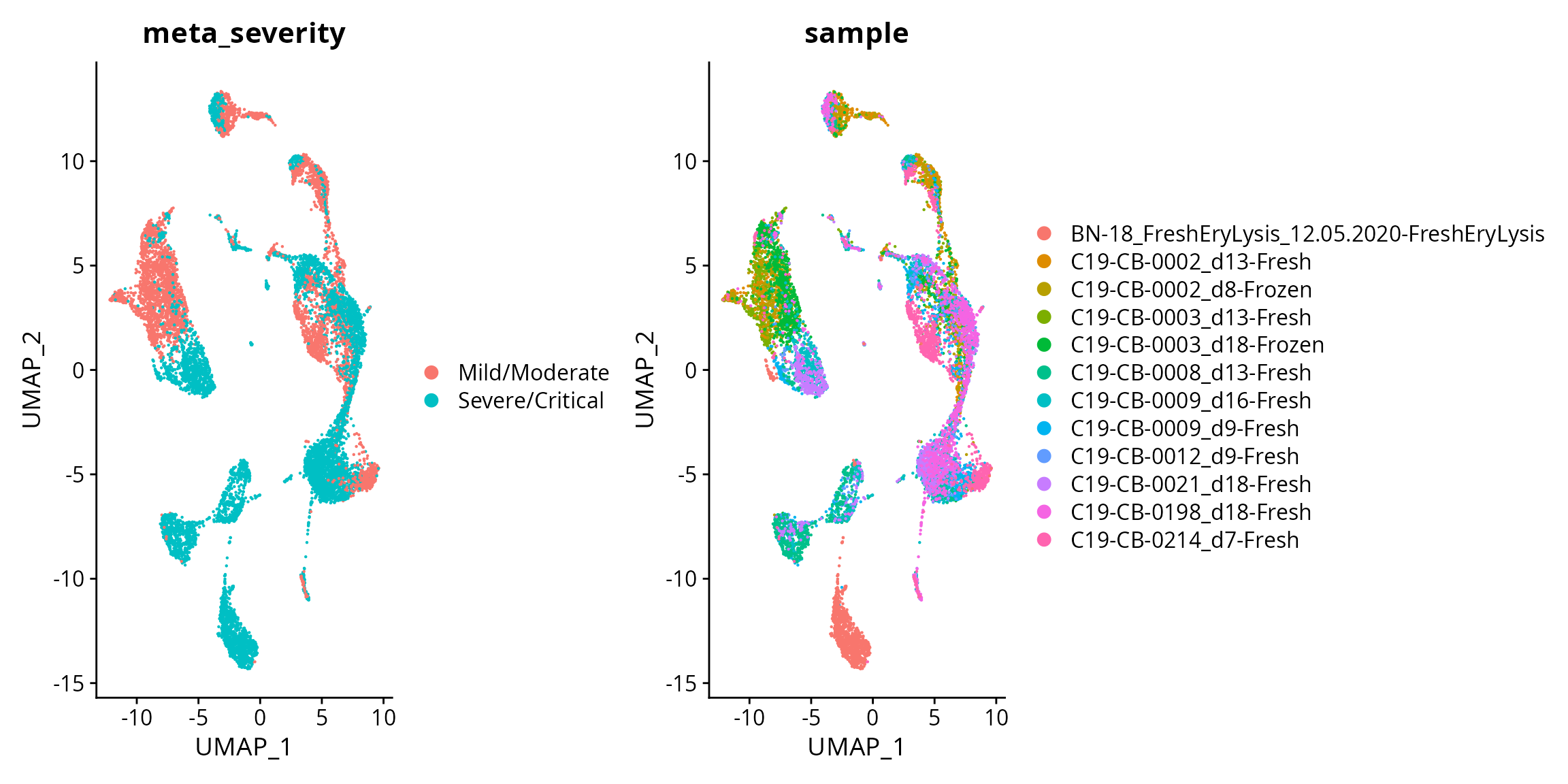
Interpretation:
Are the cells from mild/moderate and severe/critical patients easy or difficult to distinguish?
3. What insights can we gain from the molecular profiles of patients to better understand about the patients?
In this workshop, we use scFeatures
to generate molecular representation for each patient. The molecular
representation is interpretable and hence facilitates downstream
analysis of the patient. Overall, scFeatures generates features across
six categories representing different molecular views of cellular
characteristics. These include:
- i) cell type proportions
- ii) cell type specific gene expressions
- iii) cell type specific pathway expressions
- iv) cell type specific cell-cell interaction (CCI) scores
- v) overall aggregated gene expressions
- vi) spatial metrics
The different types of features constructed enable a more comprehensive
multi-view understanding of each patient from a matrix of genes x
cells.
3.1 Checking the data
Inspect the number of cells in each patient sample, as well as the number of cells in each cell type.
Discussion:
Is there any sample or cell types you should remove from the data?
table(data$sample)
#>
#> BN-18_FreshEryLysis_12.05.2020-FreshEryLysis
#>                                         1000
#>                        C19-CB-0002_d13-Fresh
#>                                         1000
#>                        C19-CB-0002_d8-Frozen
#>                                         1000
#>                        C19-CB-0003_d13-Fresh
#>                                         1000
#>                       C19-CB-0003_d18-Frozen
#>                                         1000
#>                        C19-CB-0008_d13-Fresh
#>                                         1000
#>                        C19-CB-0009_d16-Fresh
#>                                         1000
#>                         C19-CB-0009_d9-Fresh
#>                                          938
#>                         C19-CB-0012_d9-Fresh
#>                                          741
#>                        C19-CB-0021_d18-Fresh
#>                                         1000
#>                        C19-CB-0198_d18-Fresh
#>                                         1000
#>                         C19-CB-0214_d7-Fresh
#>                                         1000
table(data$celltype)
#>
#>            B    CD14 Mono    CD16 Mono        CD4 T        CD8 T           DC
#>          654         2617          314         2162          725          128
#>           DN          gdT         HSPC          ILC intermediate         MAIT
#>           14          156           19            1          232          156
#>         MAST   Neutrophil           NK          NKT       Plasma     Platelet
#>            8         2008         1189          811          204          134
#>          RBC   unassigned
#>            1          146
Discussion:
After running the process_data function, are there still
any patient samples or cell types that you should remove from the
data?
3.1 Creating molecular representations of patients
All the feature types can be generated in one line of code. This runs
the function using default settings for all parameters, for more
information, type ?scFeatures.
Given that this step may take up to 20 minutes, we have already
generated the result and saved it in the
intermediate_result folder. You could skip this step and
proceed to the next step for the purposes of this workshop.
# Here we label the samples using the severity, such as it is easier later on to retrieve the severity outcomes of the samples.
data$sample <- paste0(data$sample, "_cond_" , data$meta_severity)

# scfeatures uses the log normalised data
scfeatures_result <- scFeatures(data  = data@assays$RNA@data , sample = data$sample, celltype = data$celltype , ncores = 12)
3.2 Visualising and exploring scFeatures output
We have generated a total of 13 feature types and stored them in a
list. All generated feature types are stored in a matrix of samples by
features.
For example, the first list element contains the feature type
“proportion_raw”, which contains the cell type proportion features for
each patient sample. We could print out the first 5 columns and first 5
rows of the first element to see.
scfeatures_result <- readRDS("~/intermediate_result/scfeatures_result_schulte_12patients.rds")

# we have generated a total of 13 feature types
names(scfeatures_result)
#>  [1] "proportion_raw"     "proportion_logit"   "proportion_ratio"
#>  [4] "gene_mean_celltype" "gene_prop_celltype" "gene_cor_celltype"
#>  [7] "pathway_gsva"       "pathway_mean"       "pathway_prop"
#> [10] "CCI"                "gene_mean_bulk"     "gene_prop_bulk"
#> [13] "gene_cor_bulk"

# each row is a sample, each column is a feature
scfeatures_result[[1]][1:5, 1:5]
#>                                                    B  CD14 Mono  CD16 Mono
#> C19-CB-0003_d13-Fresh_cond_Mild/Moderate  0.15245737 0.56870612 0.06218656
#> C19-CB-0002_d13-Fresh_cond_Mild/Moderate  0.23123123 0.27327327 0.03203203
#> C19-CB-0002_d8-Frozen_cond_Mild/Moderate  0.06700000 0.27800000 0.03000000
#> C19-CB-0003_d18-Frozen_cond_Mild/Moderate 0.03200000 0.57400000 0.13400000
#> C19-CB-0009_d9-Fresh_cond_Severe/Critical 0.01611171 0.09344791 0.00000000
#>                                                CD4 T      CD8 T
#> C19-CB-0003_d13-Fresh_cond_Mild/Moderate  0.02407222 0.02407222
#> C19-CB-0002_d13-Fresh_cond_Mild/Moderate  0.06006006 0.05205205
#> C19-CB-0002_d8-Frozen_cond_Mild/Moderate  0.04600000 0.06200000
#> C19-CB-0003_d18-Frozen_cond_Mild/Moderate 0.01700000 0.03600000
#> C19-CB-0009_d9-Fresh_cond_Severe/Critical 0.33941998 0.05263158
Once the features are generated, you may wish to visually explore the features. For example, with cell type specific gene expression score, a volcano plot would provide more direct insight than a matrix of values.
data <- scfeatures_result$gene_mean_celltype
# this transposes the data
# in bioinformatics conversion, features are stored in rows
# in statistics convention, features are stored in columns
data <- t(data)

# pick CD14 Mono as an example cell type
data <- data[ grep("CD14", rownames(data)), ]
condition  <- unlist( lapply( strsplit( colnames(data), "_cond_"), `[`, 2))
condition <- data.frame(condition = condition )
design <- model.matrix(~condition, data = condition)
fit <- lmFit(data, design)
fit <- eBayes(fit)
tT <- topTable(fit, n = Inf)
tT$gene <- rownames(tT)
p <- ggplot( tT , aes(logFC,-log10(P.Value) , text = gene ) )+
      geom_point(aes(colour=-log10(P.Value)), alpha=1/3, size=1) +
      scale_colour_gradient(low="blue",high="red")+
      xlab("log2 fold change") + ylab("-log10 p-value") + theme_minimal()

ggplotly(p)
To accommodate for this need, scFeatures contains a function
run_association_study_report that enables the user to
readily visualise and explore all generated features with one line of
code.
Note, because this function knits a HTML file, please paste the following command in the console and run it there.
# specify a folder to store the html report. Here we store it in the current working directory.
output_folder <-  getwd()
run_association_study_report(scfeatures_result, output_folder )
3.3 Are the generated features sensible?
Discussion:
Using the HTML, we can look at some of the critical thinking questions that a researcher would ask about the generated features. These questions are exploratory and there is no right or wrong answer.
- Do the generated features look reasonable?
- Which cell type(s) would you like to focus on at your next stage of
analysis?
- Which feature type(s) would you like to focus on at your next stage
of analysis?
- Are the conditions in your data relatively easy or difficult to distinguish?
4. How can I leverage the molecular representation of patients to classify disease outcome?
Now that we have generated the patient representation, in this section we will examine a useful case study of using the representation to perform disease outcome classification.
4.1 Building classification model
In this workshop we use the classifyR package to build a classification model. It provides an implementation of a typical framework for classification, including a function that performs repeated cross-validation with one line of code.
We will build a classification model for each feature type.
# First clean the column names
for(i in 1:length(scfeatures_result)){
  names(scfeatures_result[[i]]) <-  make.names(names(scfeatures_result[[i]]))
}

# obtain the patient outcome, which is stored in the rownames of each matrix
outcome = scfeatures_result[[1]] %>% rownames %>% strsplit("_cond_") %>% sapply(function(x) x[2])
Recall in the previous section that we have stored the 13 feature types matrix in a list. Instead of manually retrieving each matrix from the list to build separate models, classifyR can directly take a list of matrices as an input and run repeated cross-validation model on each matrix individually.
Below, we run 5 repeats of 2 folds cross-validation (to save time).
classifyr_result = crossValidate(scfeatures_result,
                                 outcome,
                                 classifier = "kNN",
                                 nFolds = 2,
                                 nRepeats = 5,
                                 nCores = 5 )
4.2 Visualising the classification performance
To examine the classification model performance, we first need to specify a metric to calculate. Here, we calculate the balanced accuracy.
classifyr_result <- readRDS("~/intermediate_result/classifyr_result_knn.rds")

classifyr_result <- lapply(classifyr_result, function(x) calcCVperformance(x, performanceType = "Balanced Accuracy"))
Format the output and visualise the accuracy using boxplots.
accuracy_knn_balanced_accuracy  <- performancePlot(classifyr_result) + theme(axis.text.x = element_text(angle = 45, vjust = 1, hjust=1)) # make the x-axis label 45 degree so it's easier to read

accuracy_knn_balanced_accuracy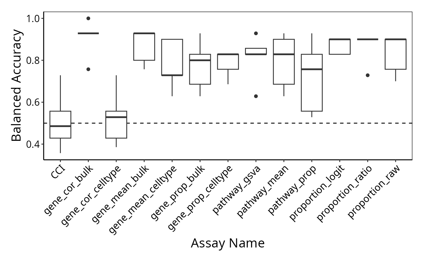
Interpretation:
Based on the classification performance, which feature type would you like to focus on at your next stage of analysis?
4.3 What features are important for disease outcome prediction?
Recall that we built 5 repeats of 2-fold cross-validation models. This means for each feature type, we have obtained a total of 10 models. Therefore, to answer what features are important in the modelling, we first need to examine whether the rankings (or the importance) of each feature in each model (within each feature type) are the same.
To give an example, we use the feature type “gene_mean_celltype” and look at the overlap between the top 20 ranked features in the 10 models.
# look at the list of models
names(classifyr_result)
#>  [1] "proportion_raw.kNN.t-test"     "proportion_logit.kNN.t-test"
#>  [3] "proportion_ratio.kNN.t-test"   "gene_mean_celltype.kNN.t-test"
#>  [5] "gene_prop_celltype.kNN.t-test" "gene_cor_celltype.kNN.t-test"
#>  [7] "pathway_gsva.kNN.t-test"       "pathway_mean.kNN.t-test"
#>  [9] "pathway_prop.kNN.t-test"       "CCI.kNN.t-test"
#> [11] "gene_mean_bulk.kNN.t-test"     "gene_prop_bulk.kNN.t-test"
#> [13] "gene_cor_bulk.kNN.t-test"

# pick the fourth model, which is on the feature type gene mean celltype
gene_mean_celltype <- classifyr_result[[4]]

data_list <- gene_mean_celltype@rankedFeatures
data_list <- lapply(data_list , function(df) {
  df[, 2][1:20]
})

names(data_list) <- paste0("Model", 1:10)
# Create the UpSet plot
upset_plot <- upset(fromList(data_list), order.by = "freq", nsets = 10)

# Display the plot
upset_plot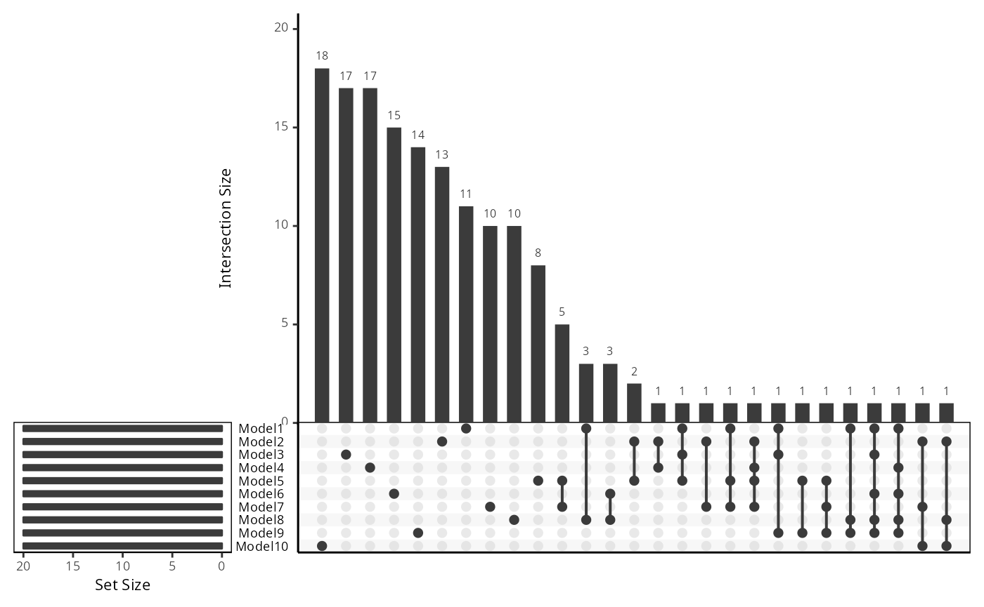
Discussion:
Based on the upset plot, is the top ranked features consistent?
This also leads to the next question, how should we determine the final set of top features to focus on?
Here, we use the mean scores across the folds to calculate the final set of top features.
top_features  <- lapply(1:10, function(x){
  thismodel <- gene_mean_celltype@rankedFeatures[[x]]
  thismodel$rank <- 1:nrow(thismodel)
  thismodel <- thismodel[sort(rownames(thismodel)), ]
  thismodel$model <- x
  thismodel
})

top_features <- as.data.frame( do.call(rbind, top_features ) )

top_features <- top_features %>% group_by(feature) %>% dplyr::summarise(rank = mean(rank)) %>% arrange(rank)

print(head(top_features,10))
#> # A tibble: 10 × 2
#>    feature               rank
#>    <chr>                <dbl>
#>  1 Neutrophil..SNX3      108.
#>  2 gdT..SATB1            113.
#>  3 Neutrophil..CAST      129.
#>  4 Neutrophil..ALOX5AP   130
#>  5 Neutrophil..SH3BGRL3  147.
#>  6 Neutrophil..FCER1G    153.
#>  7 Neutrophil..PRR13     156.
#>  8 Neutrophil..GRN       193.
#>  9 Neutrophil..CDC42     216.
#> 10 Neutrophil..YWHAB     226.
Discussion:
Explore the ranks of the features. Which cell type(s) would you like to focus on at your next stage of analysis ?
4.4 Is the prediction consistent across the feature types
Given we build prediction model for each of the feature type, we can examine whether the prediction from each feature type is consistent.
# looking at one repeat
data_list <- lapply( 1:13 , function(i) {
  prediction <- classifyr_result[[i]]@predictions
  prediction <- prediction[prediction$permutation == 1, ]$class
  prediction <- as.data.frame(prediction)
})

data_list <- do.call( cbind, data_list)
colnames(data_list)  <- names(classifyr_result)


  # count the number of times each row is labeled as "Mild/Moderate"
counts <- apply(data_list  == "Mild/Moderate", 1, sum)

# calculate the percentage of times each row is labeled as "Mild/Moderate"
percentages <- counts / ncol(data_list) * 100

patient <- unlist ( lapply ( strsplit ( classifyr_result[[1]]@originalNames, "_cond_")  , `[` , 1) )
condition <-  unlist ( lapply ( strsplit ( classifyr_result[[1]]@originalNames, "_cond_")  , `[` , 2) )
consistency <- data.frame(patient = patient  ,
                          condition = condition,
                          percentages_mildmoderate = percentages )
rownames(consistency) <- NULL
consistency
#>                                         patient       condition
#> 1                         C19-CB-0003_d13-Fresh   Mild/Moderate
#> 2                         C19-CB-0002_d13-Fresh   Mild/Moderate
#> 3                         C19-CB-0002_d8-Frozen   Mild/Moderate
#> 4                        C19-CB-0003_d18-Frozen   Mild/Moderate
#> 5                          C19-CB-0009_d9-Fresh Severe/Critical
#> 6                          C19-CB-0012_d9-Fresh Severe/Critical
#> 7                         C19-CB-0008_d13-Fresh Severe/Critical
#> 8                         C19-CB-0009_d16-Fresh Severe/Critical
#> 9                         C19-CB-0021_d18-Fresh Severe/Critical
#> 10                        C19-CB-0198_d18-Fresh Severe/Critical
#> 11                         C19-CB-0214_d7-Fresh   Mild/Moderate
#> 12 BN-18_FreshEryLysis_12.05.2020-FreshEryLysis Severe/Critical
#>    percentages_mildmoderate
#> 1                 92.307692
#> 2                 92.307692
#> 3                 38.461538
#> 4                 53.846154
#> 5                  0.000000
#> 6                 23.076923
#> 7                 84.615385
#> 8                 84.615385
#> 9                  7.692308
#> 10                 0.000000
#> 11                 7.692308
#> 12                 7.692308

# can also do it visually in one line via the function:
samplesMetricMap(classifyr_result)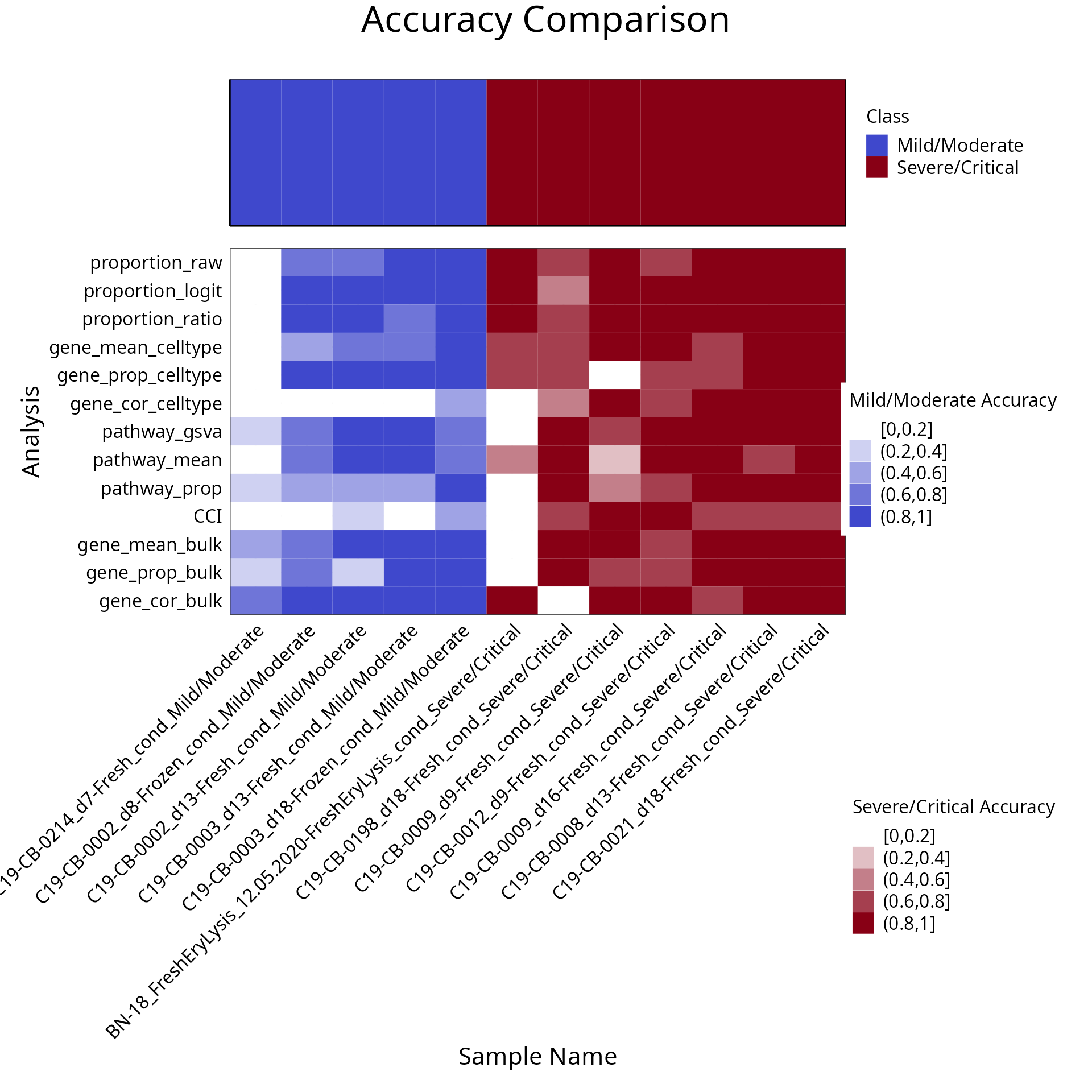
#> TableGrob (2 x 1) "arrange": 2 grobs
#>   z     cells    name                grob
#> 1 1 (2-2,1-1) arrange      gtable[layout]
#> 2 2 (1-1,1-1) arrange text[GRID.text.678]
Discussion:
Would ensemble learning using all feature types improve prediction performance compared to using the individual feature type ?
5. How do we ensure the model reliably predicts disease outcome ?
In this section we take a detailed look at the model performance. In particular, a number of factors may affect the classification performance, such as the choice of classification algorithm.
5.1 Do the results change with different classification algorithms?
classifyR provides an implementation of a number of commonly used
classification algorithms, including:
- randomForest
- DLDA
- kNN
- GLM
- elasticNetGLM
- SVM
- NSC
- naiveBayes
- mixturesNormals
- CoxPH
- CoxNet
- randomSurvivalForest
- XGB
classifyr_result = crossValidate(scfeatures_result,
                                 outcome,
                                 classifier = "naiveBayes",
                                 nFolds = 2,
                                 nRepeats = 5,
                                 nCores = 5 )
Compare the accuracy obtained from the different algorithms.
classifyr_result <- readRDS("~/intermediate_result/classifyr_result_naivebayes.rds")

accuracy_naivebayes_balanced_accuracy <- performancePlot(classifyr_result) + theme(axis.text.x = element_text(angle = 45, vjust = 1, hjust=1))

accuracy_naivebayes_balanced_accuracy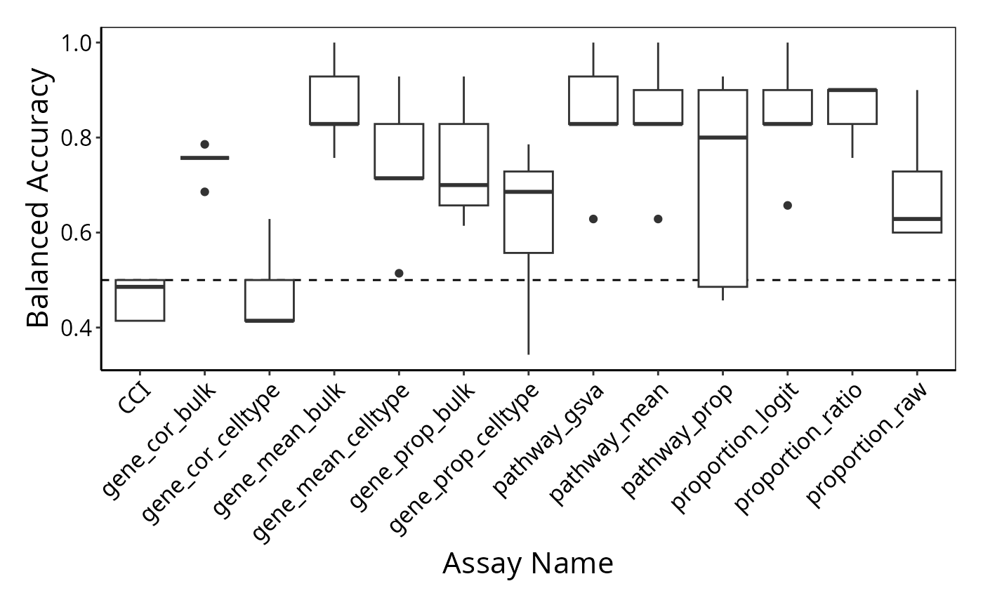
5.2 Do the results change with different evaluation metrics?
Here we calculate accuracy instead of balanced accuracy. Inspect the difference in performance.
accuracy_naivebayes_accuracy  <- performancePlot(classifyr_result , metric ="Accuracy" ) + theme(axis.text.x = element_text(angle = 45, vjust = 1, hjust=1))

accuracy_naivebayes_accuracy 
Compare the performance on the same plot
ggpubr::ggarrange(plotlist = list(accuracy_knn_balanced_accuracy,
                                  accuracy_naivebayes_balanced_accuracy,
                                  accuracy_naivebayes_accuracy),
                  ncol=3)
5.3 Is the model generalisable?
Generalisable means whether the model can have good performance when tested on an independent dataset.
Here, we use the model built on the Schulte-Schrepping dataset to test on the Wilk dataset. The Wilk data is obtained from Wilk et al. 2022. We sampled 12 patients with mild/moderate and severe/critical conditions.
data <- readRDS("~/toy_data/wilk_12patients.rds")First visualise the data.
data <- NormalizeData( data)

data <-  FindVariableFeatures(data )
data <- ScaleData(data, features = rownames(data) )
data <- RunPCA(data)
data <- FindNeighbors(data, dims = 1:10)
data <- FindClusters(data, resolution = 0.5)
#> Modularity Optimizer version 1.3.0 by Ludo Waltman and Nees Jan van Eck
#>
#> Number of nodes: 9029
#> Number of edges: 306374
#>
#> Running Louvain algorithm...
#> Maximum modularity in 10 random starts: 0.9119
#> Number of communities: 13
#> Elapsed time: 0 seconds
data  <- RunUMAP(data , dims = 1:10)
DimPlot(data, reduction = "umap", group.by = "meta_severity") +  DimPlot(data, reduction = "umap", group.by = "sample")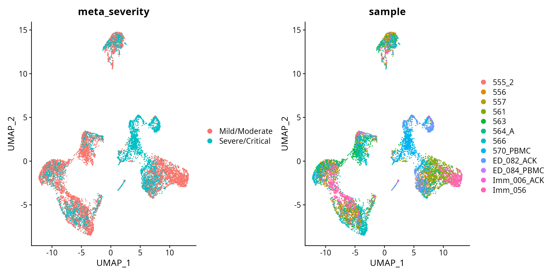
# Here we label the samples using the severity, such as it is easier later on to retrieve the severity outcomes of the samples.
data$sample <- paste0(data$sample, "_cond_" , data$meta_severity)

data <- process_data(data)

table(data$celltype)
table(data$sample)


data <- data[, -c(which(data$sample %in% c("ED_084_PBMC_cond_Severe/Critical",
                                           "Imm_006_ACK_cond_Mild/Moderate"))) ]
data <- data[, -c(which(data$celltype %in% c("DC", "DN", "gdT",  "HSPC" , "MAIT" , "MAST", "RBC")))]

scfeatures_result_wilk <- scFeatures(data, ncores = 12)
Here we have provided the constructed scFeatures result for the Wilk dataset.
scfeatures_result_schulte <- readRDS("~/intermediate_result/scfeatures_result_schulte_12patients.rds")

scfeatures_result_wilk <- readRDS("~/intermediate_result/scfeatures_result_wilk_12patients.rds" )

scfeatures_result_wilk <- scfeatures_result_wilk[ names(scfeatures_result_schulte )]


# in order to train and test two different datasets, need to make sure the features are the same
# pick the common features
new_list <- lapply( 1:length(scfeatures_result_schulte), function(i){
  common_features <- intersect(colnames( scfeatures_result_schulte[[i]]) ,
                               colnames( scfeatures_result_wilk[[i]]))
  new_schulte <-  scfeatures_result_schulte[[i]][, common_features]
  new_wilk <- scfeatures_result_wilk[[i]][, common_features]
  list(new_schulte, new_wilk)
})

# format the features
new_scfeatures_result_schulte <- lapply(new_list, `[[`, 1)
new_scfeatures_result_wilk <- lapply(new_list, `[[`, 2)

names(new_scfeatures_result_schulte) <- names(scfeatures_result_schulte)
names(new_scfeatures_result_wilk) <- names(scfeatures_result_wilk)


# obtain the outcome, which is stored in the rownames of ech matrix
outcome_schulte = scfeatures_result_schulte[[1]] %>% rownames %>% strsplit("_cond_") %>% sapply(function(x) x[2])

outcome_wilk = scfeatures_result_wilk[[1]] %>% rownames %>% strsplit("_cond_") %>% sapply(function(x) x[2])
names(outcome_wilk) <- rownames(scfeatures_result_wilk[[1]])
Building the model on Schulte-Schrepping dataset features and testing on the Wilk dataset.
# First clean the column names
for(i in 1:length(new_scfeatures_result_schulte)){
  names(new_scfeatures_result_schulte[[i]]) <-  make.names( names(new_scfeatures_result_schulte[[i]]) )
}


# First clean the column names
for(i in 1:length(new_scfeatures_result_wilk)){
  names(new_scfeatures_result_wilk[[i]]) <-  make.names( names(new_scfeatures_result_wilk[[i]]) )
}


# for each feature type, identify the best model and use the best model to predict on Wilk
result_generalisability <- NULL

for( i in c(1:length( new_scfeatures_result_schulte )) ){

  model <- train(x = new_scfeatures_result_schulte[[i]] ,outcomeTrain = outcome_schulte,
                 performanceType = "Balanced Accuracy", classifier =  "DLDA" )
  prediction  <- predict( model , new_scfeatures_result_wilk[[i]])
  truth <-  outcome_wilk[rownames(prediction)]
  prediction <- ifelse(prediction$`Mild/Moderate` > 0.5, "Mild/Moderate", "Severe/Critical" )
  temp <- calcExternalPerformance( factor(truth) , factor(prediction),
                                   performanceType = c("Balanced Accuracy"))
  temp <- data.frame(balanced_accuracy = temp,
                     featuretype = names(new_scfeatures_result_schulte)[[i]] )
  result_generalisability <- rbind(result_generalisability,   temp)
}
Visualise the accuracy using boxplots.
result_generalisability$balanced_accuracy <- round( result_generalisability$balanced_accuracy, 2)


result_generalisability$featuretype <- factor(  result_generalisability$featuretype , levels = c( result_generalisability$featuretype))

ggplot( result_generalisability, aes(x = featuretype , y = balanced_accuracy, fill = featuretype ) ) + geom_col()+ theme(axis.text.x = element_text(angle = 45, vjust = 1, hjust=1)) + ylim(0,1) + scale_fill_tableau(palette = "Tableau 20") +
  geom_text(aes(label = balanced_accuracy), vjust = -0.5)
Discussion:
Examine the classification accuracy and comment on the generalisability of the model.
Final discussion:
How good do you think our model is? What parts of the workflow could you change to improve the results?