library(ClassifyR)
library(ggplot2)3 Procedure 2: Multi-view classifiability evaluation
3.1 Introduction
Procedure 2 aims to investigate whether individual data views serve as the best predictors of breast cancer outcomes, or if integrating multiple views improve predictive accuracy. A view could be an omics assay or a particular metafeature generated from a particular data set.
In this analysis, the METABRIC breast cancer data set will be used for 165 samples with no detected lymph node metastasis. Different omics assays and pre-generated views will be utilised:
- Clinical: Contains the outcome of interest (recurrence-free survival) as well as covariates that could predict it, such as tumour size and grade.
- RNA abundance: This was measured by microarrays. Quantile normalisation and prove reannotation was made by cBioPortal. Top 2000 highly-variable genes are used for illustration.
- Imaging mass cytometry: Complementary to RNA, this assay gives the protein abundances for a small panel of 39 proteins. This is the basis of:
- Type Proportions: Using annotated cell types, the proportion of each cell type in each patient sample.
- Type Protein Mean: For each cell type, the average abundance of each feature in each sample.
- Type Pairs Colocated: For each pair of cell types, a score of association using their X and Y coordinates based on L curve.
- Colocated in Regions: k-means clustering-based definition of regions and spatial association within them.
- Proportion of Parent: Based on HOPACH hierarchical clustering, the proportion of a cell type to its parent type.
3.2 Setting up the environment and data objects
1. Load the R packages into the R environment
Timing ~ 6.6s
ClassifyR is used to perform all the demonstrated analyses below.
2. Import preprocessed datasets for analysis
Timing ~ 0.055s
METABRIC <- readRDS("data/procedure2/METABRICviews.rds")This command reads in the list of 7 preprocessed assays and views mentioned previously. They are named “clinical”, “RNA Microarray”, “Type Proportions”, “Type Protein Mean”, “Type Pairs Colocated”, “Colocated in Regions” and “Proportion of Parent”. They respectively contain 30, 2000, 22, 858, 484, 10 and 55 features for each of the 165 samples.
3.3 Model Building and Evaluation
Here, models will be built by 3 different methods of assay and view integrations: step 3 - individual assays, step 4 - merging assays and step 5 - prevalidation.
3. Individual Assays
Timing ~ 82s
set.seed(1)
usefulFeatures <- c("Breast.Tumour.Laterality", "ER.Status", "Inferred.Menopausal.State",
                    "Grade", "Size", "Stage")
coxCV <- crossValidate(METABRIC, c("timeRFS", "eventRFS"), selectionMethod = "CoxPH", classifier = "CoxNet",
                       nCores = 8, extraParams = list(prepare = list(useFeatures = list(clinical = usefulFeatures))))
The set.seed(1) command ensures that any subsequent operations involving randomness yield consistent results across runs.
The next command selects only the biologically relevant features in the clinical data to be used later for model building, as there are arbitrary sample identifiers, dates and other non-biological information which should not be used
The crossValidate function is then used to perform 5-fold cross-validation for 20 repeats, fitting a penalised Cox proportional hazards model to each assay individually. 20 CPU cores are used for parallel processing to speed up classification. The type of classifier, number of folds, repeats and cores used can be adjusted as wished for different analyses. The outcomes here are timeRFS and eventRFS, 2 columns from METABRIC[["clinical"]].
Timing ~ 1.5s
performancePlot(coxCV, orderingList = list("Assay Name" = "performanceDescending")) +
    theme(axis.text.x = element_text(angle = 45, vjust = 1, hjust = 1))
Warning in .local(results, ...): C-index not found in all elements of results.
Calculating it now.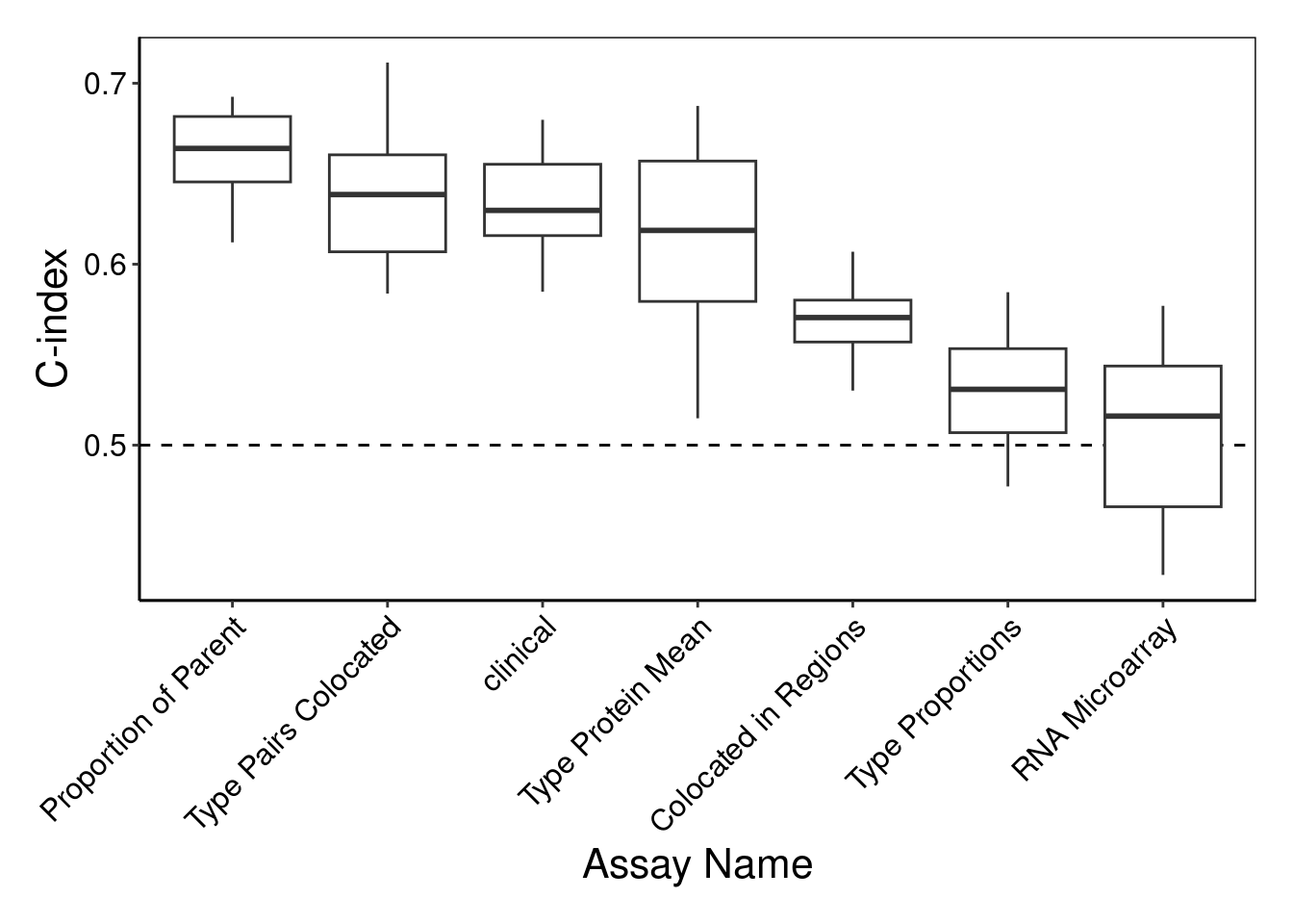
png
  2
This command generates a side-by-side boxplot of C-index for each individual assay by performancePlot to compare their classification performance. The most accurate view is Proportion of Parent, but interestingly, using just the freely available clinical data attains a similar performance. Further, the protein assay views also performed surprisingly well despite having about a hundred times less features to use than RNA does.
Timing ~ 22s
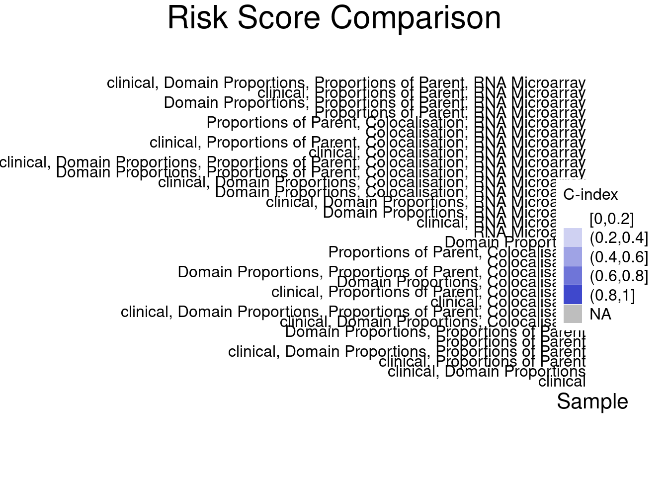
samplesMetricMap(coxCV, showXtickLabels = FALSE)Warning in .local(results, ...): Sample C-index not found in all elements of
results. Calculating it now.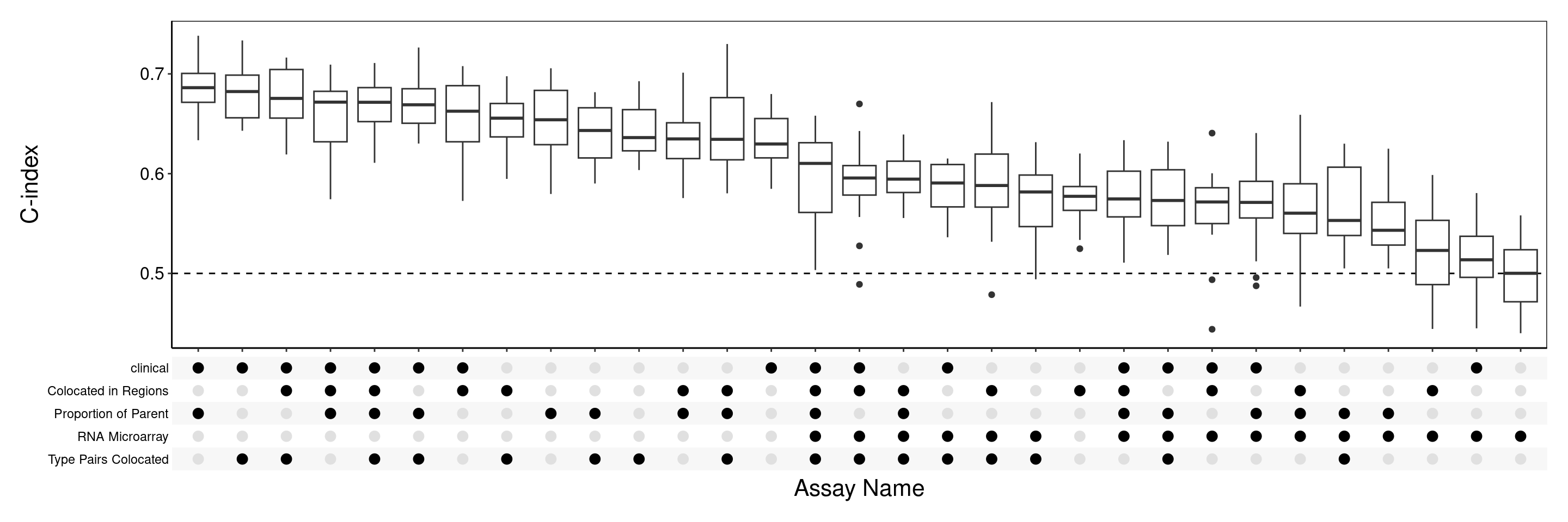
TableGrob (2 x 1) "arrange": 2 grobs
  z     cells    name                grob
1 1 (2-2,1-1) arrange      gtable[layout]
2 2 (1-1,1-1) arrange text[GRID.text.508]
png
2 4. Merged Assays
Timing ~ 29mins
Note: Type Protein Mean and Type Proportions have been removed for the following analysis to save run time.
set.seed(1)
xOrder <- list("Assay Name" = "performanceDescending")
merge <- c("clinical", "Domain Proportions", "Proportions of Parent", "Colocalisation", "RNA Microarray")
coxMergeCV <- crossValidate(METABRIC[merge], c("timeRFS", "eventRFS"), multiViewMethod = "merge", extraParams = list(prepare = list(useFeatures = list(clinical = usefulFeatures))), selectionMethod = "CoxPH", classifier = "CoxNet", nCores = 8)
performancePlot(coxMergeCV, orderingList = list("Assay Name" = "performanceDescending"))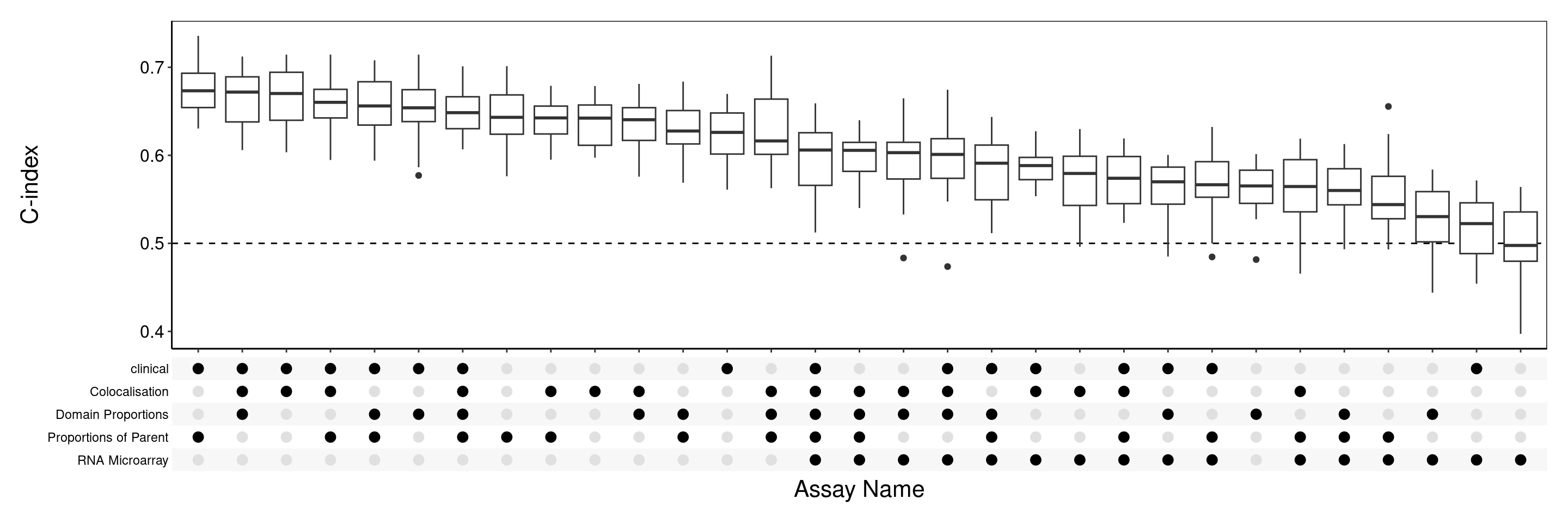
png
2 The 3 commands used here are the same as for individual assays in step 3, with the only difference being the merge combination method used for the multiViewMethod argument in the second command to concatenate the independently selected features in each view. Other multiVewMethods include prevalidation and PCA. The produced plot suggests that combining clinical data with imaging mass cytometry views can improve performance. Specifically, the best performing combination used clinical, Colocated in Regions and Type Pairs Colocated to achieve a C-index which surpasses Proportion of Parent, the best performing individual assay. Hence, integrating multiple views have successfully improved prediction accuracy.
Timing ~ 95s
samplesMetricMap(coxMergeCV, showXtickLabels = FALSE)Warning in .local(results, ...): Sample C-index not found in all elements of
results. Calculating it now.