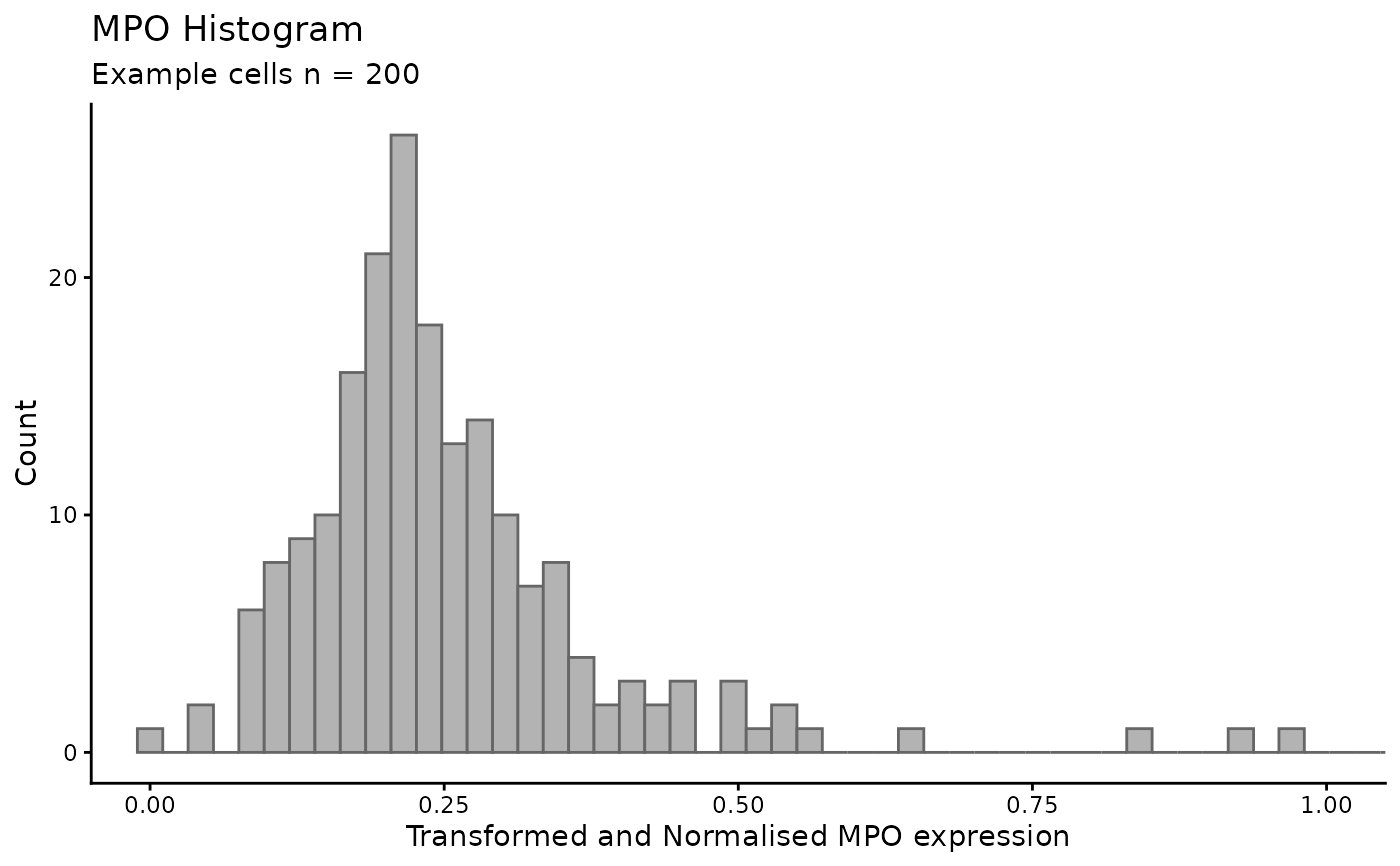
Plot marker intensity with optional GMM fit — plot_ct_marker

Visualizes a marker distribution, optionally with a two-component GMM fit and cutoff overlays. Useful for QC and comparing marker behavior across groups.

Usage

plot_ct_marker_intensity(
  spe,
  marker,
  subtitle,
  binwidth = NULL,
  label_col = NULL,
  cell_type = NULL,
  do_fit = TRUE,
  cutoff_method = "equal_posteriors",
  gmm_model_names = NULL,
  label_levels = NULL,
  label_colors = NULL,
  drop_levels = FALSE,
  assay_name = "exprs"
)

Arguments

spe: A `SpatialExperiment`/`SingleCellExperiment`.
marker: Marker name to plot (must match a row in the assay).
subtitle: Subtitle for the plot.
binwidth: Histogram bin width. If NULL, uses range/100.
label_col: Optional column in `colData(spe)` used to subset to a specific cell type and to color the histogram.
cell_type: Optional cell type value to subset when `label_col` is set.
do_fit: Logical; fit a 2-component GMM and draw the components.
cutoff_method: Passed to [fit_gmm_2()].
gmm_model_names: Passed to [fit_gmm_2()].
label_levels: Optional character vector of label levels to enforce for legend consistency.
label_colors: Optional named or unnamed vector of colors to use for the label levels. If provided alongside `label_levels`, lengths must match.
drop_levels: Logical; if FALSE, keep unused levels in the legend. Default FALSE.
assay_name: Assay name to pull values from. Default "exprs".

Value

A `ggplot` object.

Examples

data("cytoGateR_example", package = "cytoGateR")
spe <- cytoGateR_example[, seq_len(min(200L, ncol(cytoGateR_example)))]
plot_ct_marker_intensity(
  spe,
  marker = rownames(spe)[1],
  subtitle = "Example cells",
  do_fit = FALSE
)