Overview
Tree gating can identify high-confidence reference cells while leaving ambiguous cells unassigned. This vignette uses the stored core_group labels to train a weighted k-nearest-neighbour classifier and predict the remaining cells.
The example uses one complete image and reduced cross-validation settings to remain suitable for package checks.
library(cytoGateR)
data("cytoGateR_example", package = "cytoGateR")

image_ids <- SummarizedExperiment::colData(cytoGateR_example)$image_name
spe <- cytoGateR_example[, image_ids == image_ids[1L]]
table(SummarizedExperiment::colData(spe)$core_group)
      Bcell     BnTcell         CD4         CD8     Myeloid  Neutrophil
        236         337         227         206         108          12
Plasma_cell      Stroma        Treg       Tumor  Unassigned
         40          71         125          16        2985
Train a weighted kNN reference
Only cells with a known core_group label are used during reference cleaning. The "Unassigned" cells are retained for subsequent prediction.
knn_reference <- train_custom_knn(
  spe,
  label_col = "core_group",
  assay_name = "exprs",
  unknown_label = "Unassigned",
  features = c("CD3e", "CD20", "CD4", "CD8a"),
  cv_folds = 2,
  repeats = 1,
  agreement_thresh = 0.5,
  k = 3,
  method = "pearson",
  seed = 1,
  BPPARAM = BiocParallel::SerialParam()
)
The returned object contains a cleaned reference and cross-validated probabilities for retained reference cells:
[1] "spe"             "model"           "core_prob_mat"   "agreement_rates"
[5] "features_used"
dim(knn_reference$model$reference_data)
table(knn_reference$model$reference_labels)
      Bcell     BnTcell         CD4         CD8     Myeloid  Neutrophil
        175         197         154         165          52           0
Plasma_cell      Stroma        Treg       Tumor
          6           7          24           2
Predict unassigned cells
knn_prediction <- predict_unknown_with_knn(
  knn_reference$spe,
  knn_reference,
  assay_name = "exprs",
  label_col = "cleaned_core_label",
  out_col = "knn_label_filled",
  pred_col = "knn_pred",
  unknown_label = "Unassigned",
  threshold = 0.5,
  k = 3,
  dist_method = "pearson"
)
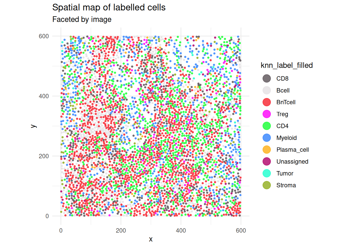
prediction_cd <- SummarizedExperiment::colData(knn_prediction$spe)
table(prediction_cd$knn_label_filled)
      Bcell     BnTcell         CD4         CD8     Myeloid Plasma_cell
        603        1369         861         502         564          66
     Stroma        Treg       Tumor  Unassigned
        106         131          59         102
summary(prediction_cd$knn_confidence)
   Min. 1st Qu.  Median    Mean 3rd Qu.    Max.     NAs
 0.3334  0.6670  1.0000  0.8771  1.0000  1.0000     782
Assemble the full probability matrix
train_custom_knn() returns probabilities for retained reference cells, while predict_unknown_with_knn() returns probabilities for predicted cells. They can be combined and aligned to the cells present in the updated object.
full_prob_mat <- rbind(
  knn_reference$core_prob_mat,
  knn_prediction$prob_mat
)
full_prob_mat <- full_prob_mat[colnames(knn_prediction$spe), , drop = FALSE]

dim(full_prob_mat)
   Min. 1st Qu.  Median    Mean 3rd Qu.    Max.
      1       1       1       1       1       1
Quantify uncertainty
The uncertainty calculation combines probability-distribution measures with a sample-aware spatial-discordance score.
uncertainty <- calculate_uncertainty(
  full_prob_mat,
  knn_prediction$spe,
  sample_col = "sample_id",
  k_spatial = 3
)
head(uncertainty)
     cell_id   entropy gini_impurity margin_uncertainty spatial_discordance
12_1    12_1 0.0000000     0.0000000          0.0000000           0.3333333
12_2    12_2 0.0000000     0.0000000          0.0000000           0.3333333
12_3    12_3 0.0000000     0.0000000          0.0000000           0.3333333
12_4    12_4 0.0000000     0.0000000          0.0000000           1.0000000
12_5    12_5 0.2763651     0.4936561          0.6662051           1.0000000
12_6    12_6 0.2764426     0.4938469          0.6667198           0.6666667
Compare labels
             v2
v1            Bcell BnTcell  CD4  CD8 Myeloid Neutrophil Plasma_cell Stroma
  Bcell         212      21    3    3      33          0           5      7
  BnTcell       256    1197  526  344      56          0          11      4
  CD4             0       0    5    0       0          0           0      0
  CD8             0       4    1   78       0          0           1      0
  Myeloid        52      30   74   39     314          0          34     45
  Neutrophil      5       0    3    1      27          0           1      8
  Plasma_cell     0       0    1    0       1          0           0      1
  Stroma          0       1    2    1       5          0           1      0
  Treg            0       5  170    0      10          0           2      0
  Tumor           0       0    0    0       1          0           0      0
  Unassigned      0       0    0    0       0          0           0      0
  Uncertain      78     111   76   36     117          0          11     41
             v2
v1            Treg Tumor Unassigned Uncertain
  Bcell          0     5          7         0
  BnTcell       80     3         29         0
  CD4            0     0          0         0
  CD8            1     0          2         0
  Myeloid        7    26         33         0
  Neutrophil     1     8          0         0
  Plasma_cell    0     0          0         0
  Stroma         0     0          1         0
  Treg          33     3          3         0
  Tumor          0     0          0         0
  Unassigned     0     0          0         0
  Uncertain      9    14         27         0
plot_labelled_cells(
  knn_prediction$spe,
  col_label = "knn_label_filled",
  image_col = "image_name"
)
Other classifiers
cytoGateR also provides random-forest and optional Torch-based deep-learning classifiers. They use the same core-label and unknown-cell workflow. The following production alternatives are not evaluated during vignette building.
rf_reference <- train_custom_randomforest(
  spe,
  label_col = "core_group",
  unknown_label = "Unassigned",
  cv_folds = 5,
  repeats = 10,
  seed = 1
)

dl_reference <- train_custom_dl(
  spe,
  label_col = "core_group",
  unknown_label = "Unassigned",
  epochs = 50,
  cv_folds = 5,
  repeats = 3,
  seed = 1
)
R version 4.6.1 (2026-06-24)
Platform: x86_64-pc-linux-gnu
Running under: Ubuntu 24.04.5 LTS

Matrix products: default
BLAS:   /usr/lib/x86_64-linux-gnu/openblas-pthread/libblas.so.3
LAPACK: /usr/lib/x86_64-linux-gnu/openblas-pthread/libopenblasp-r0.3.26.so;  LAPACK version 3.12.0

locale:
 [1] LC_CTYPE=C.UTF-8       LC_NUMERIC=C           LC_TIME=C.UTF-8
 [4] LC_COLLATE=C.UTF-8     LC_MONETARY=C.UTF-8    LC_MESSAGES=C.UTF-8
 [7] LC_PAPER=C.UTF-8       LC_NAME=C              LC_ADDRESS=C
[10] LC_TELEPHONE=C         LC_MEASUREMENT=C.UTF-8 LC_IDENTIFICATION=C

time zone: UTC
tzcode source: system (glibc)

attached base packages:
[1] stats     graphics  grDevices utils     datasets  methods   base

other attached packages:
[1] cytoGateR_0.99.0

loaded via a namespace (and not attached):
 [1] SummarizedExperiment_1.42.0 gtable_0.3.6
 [3] rjson_0.2.23                xfun_0.61
 [5] ggplot2_4.0.3               ggrepel_0.9.8
 [7] Biobase_2.72.0              lattice_0.22-9
 [9] vctrs_0.7.3                 tools_4.6.1
[11] generics_0.1.4              parallel_4.6.1
[13] stats4_4.6.1                proxy_0.4-29
[15] tibble_3.3.1                pkgconfig_2.0.3
[17] Matrix_1.7-5                RColorBrewer_1.1-3
[19] pals_1.10                   S7_0.2.2
[21] S4Vectors_0.50.3            lifecycle_1.0.5
[23] compiler_4.6.1              farver_2.1.2
[25] ggforce_0.5.0               mapproj_1.2.12
[27] codetools_0.2-20            Seqinfo_1.2.0
[29] graphlayouts_1.2.5          maps_3.4.3
[31] htmltools_0.5.9             yaml_2.3.12
[33] pillar_1.11.1               tidyr_1.3.2
[35] MASS_7.3-65                 BiocParallel_1.46.0
[37] SingleCellExperiment_1.34.0 DelayedArray_0.38.2
[39] cachem_1.1.0                dbscan_1.2.7
[41] magick_2.9.1                viridis_0.6.5
[43] abind_1.4-8                 mclust_6.1.3
[45] tidyselect_1.2.1            digest_0.6.39
[47] dplyr_1.2.1                 purrr_1.2.2
[49] labeling_0.4.3              polyclip_1.10-7
[51] fastmap_1.2.0               grid_4.6.1
[53] colorspace_2.1-4            cli_3.6.6
[55] SparseArray_1.12.3          magrittr_2.0.5
[57] S4Arrays_1.12.1             dichromat_2.0-1
[59] ggraph_2.2.2                tidygraph_1.3.1
[61] withr_3.0.3                 scales_1.4.0
[63] rmarkdown_2.32              XVector_0.52.0
[65] matrixStats_1.5.0           igraph_2.3.4
[67] otel_0.2.0                  gridExtra_2.3.1
[69] SpatialExperiment_1.22.0    memoise_2.0.1
[71] evaluate_1.0.5              knitr_1.52
[73] GenomicRanges_1.64.0        IRanges_2.46.0
[75] viridisLite_0.4.3           rlang_1.3.0
[77] Rcpp_1.1.2                  glue_1.8.1
[79] tweenr_2.0.3                BiocGenerics_0.58.1
[81] jsonlite_2.0.0              R6_2.6.1
[83] MatrixGenerics_1.24.0