Overview
This vignette demonstrates an interpretable tree-gating workflow on one complete image from cytoGateR_example. A small two-lineage marker table keeps the build fast while exercising the same functions used by larger analyses.
library(cytoGateR)
data("cytoGateR_example", package = "cytoGateR")

image_ids <- SummarizedExperiment::colData(cytoGateR_example)$image_name
spe <- cytoGateR_example[, image_ids == image_ids[1L]]
spe
class: SpatialExperiment
dim: 40 4363
metadata(0):
assays(1): exprs
rownames(40): MPO H3 ... DNA1 DNA2
rowData names(0):
colnames(4363): 12_1 12_2 ... 12_4371 12_4372
colData names(28): sample_id image_name ... KNN_P_Treg KNN_P_Tumor
reducedDimNames(0):
mainExpName: IMMUcan_2022_CancerExample_v1
altExpNames(0):
spatialCoords names(2) : cell_x cell_y
imgData names(1): sample_id
Define a lineage table
Each row defines a cell type using positive and negative protein markers. Marker columns are list-columns so that each cell type may use a different number of markers.
lineage_table <- data.frame(
  cell_type = c("Tcell", "Bcell"),
  pos_markers = I(list("CD3e", "CD20")),
  neg_markers = I(list("CD20", "CD3e"))
)
lineage_table
  cell_type pos_markers neg_markers
1     Tcell        CD3e        CD20
2     Bcell        CD20        CD3e
Fit tree-gating models
For package-build speed, the example limits each tree to one split. Larger analyses can increase max_depth and use more detailed marker definitions.
tree_result <- run_tree_gating(
  spe,
  lineage_table,
  assay_name = "exprs",
  max_depth = 1,
  min_cells = 100,
  min_score = 0.1,
  uncert_thresh = 0.25,
  workers = 1
)
The result contains the updated object, fitted trees, probability matrix, hard labels, and cleaned lineage table:
[1] "spe"           "trees"         "prob_mat"      "hard_label"
[5] "lineage_table"
head(tree_result$prob_mat)
         Tcell      Bcell
[1,] 0.2420576 0.10869472
[2,] 0.1044300 0.20919355
[3,] 0.1894045 0.19044783
[4,] 0.2154711 0.14175073
[5,] 0.2096775 0.14963792
[6,] 0.2576276 0.07941206
table(tree_result$hard_label)
    Bcell     Tcell Uncertain
      101       686      3576
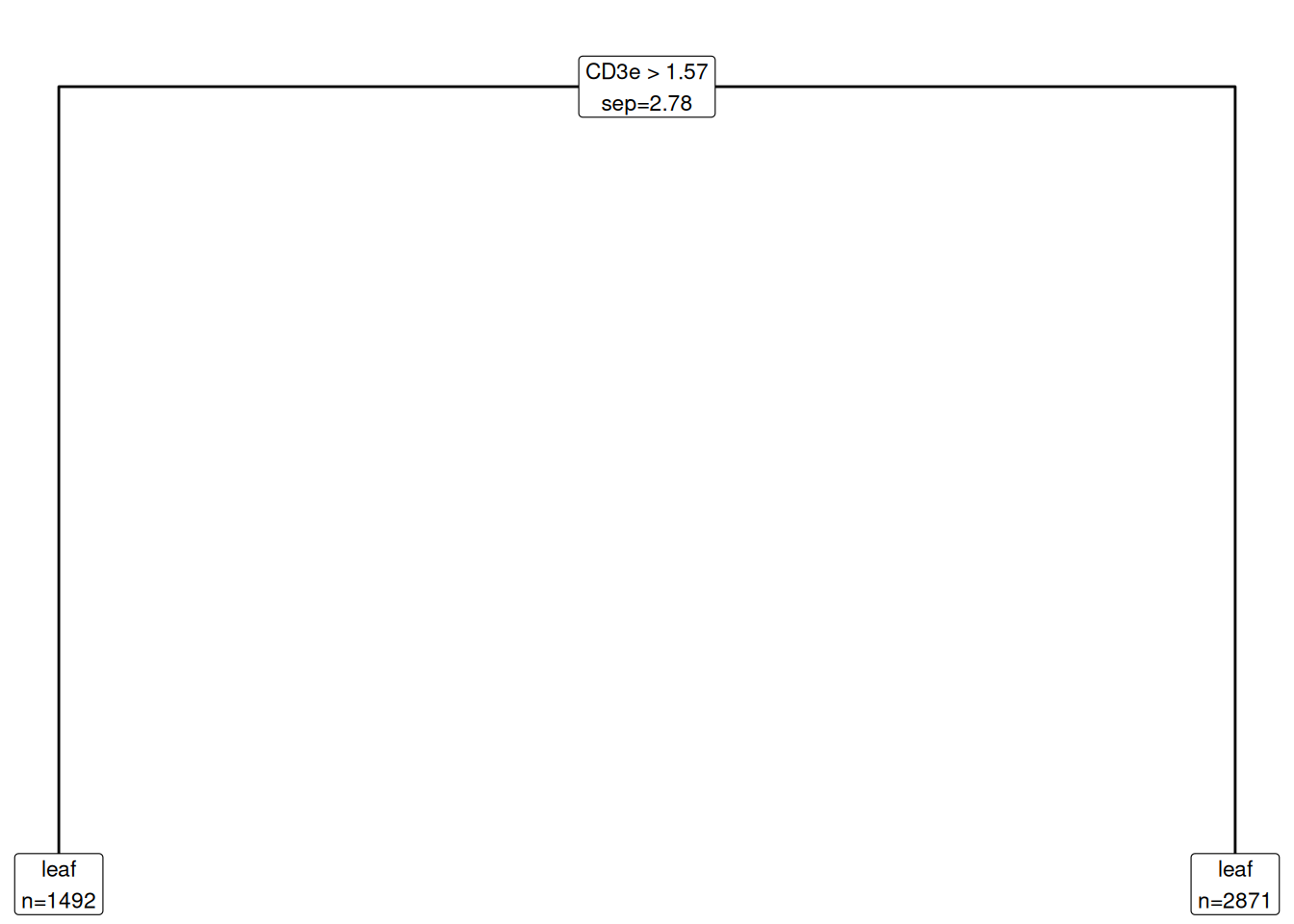
Inspect the fitted trees
[depth 0] CD3e > 1.565  (sep = 2.78, n = 4363)
 |- low
 |  [leaf] depth =1 n_cells =1492
 `- high
    [leaf] depth =1 n_cells =2871
Select high-confidence cells
apply_cutoff_labels() applies a cell-type-specific probability cutoff. A cell receives a reference label only when exactly one cell type passes its cutoff.
core_result <- apply_cutoff_labels(
  tree_result,
  cutoff_fn = function(x) stats::quantile(x, 0.95, na.rm = TRUE),
  label_col = "core_group",
  unknown_label = "Unknown"
)

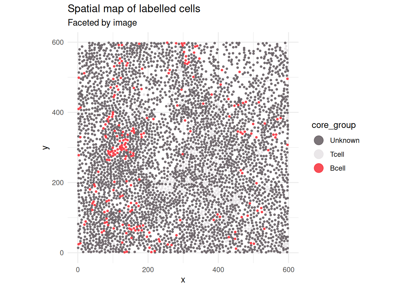
table(SummarizedExperiment::colData(core_result$spe)$core_group)
  Bcell   Tcell Unknown
    219     219    3925
Visualise expression and annotations
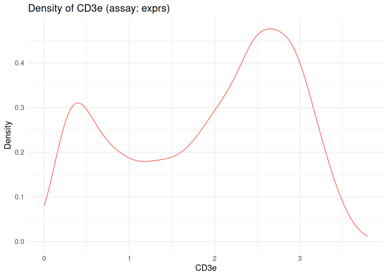
Marker distributions help assess whether the selected markers separate the expected populations.
plot_marker_density(
  core_result$spe,
  marker = "CD3e",
  assay_name = "exprs",
  image_col = "image_name"
)
The gated labels can also be displayed in spatial coordinates:
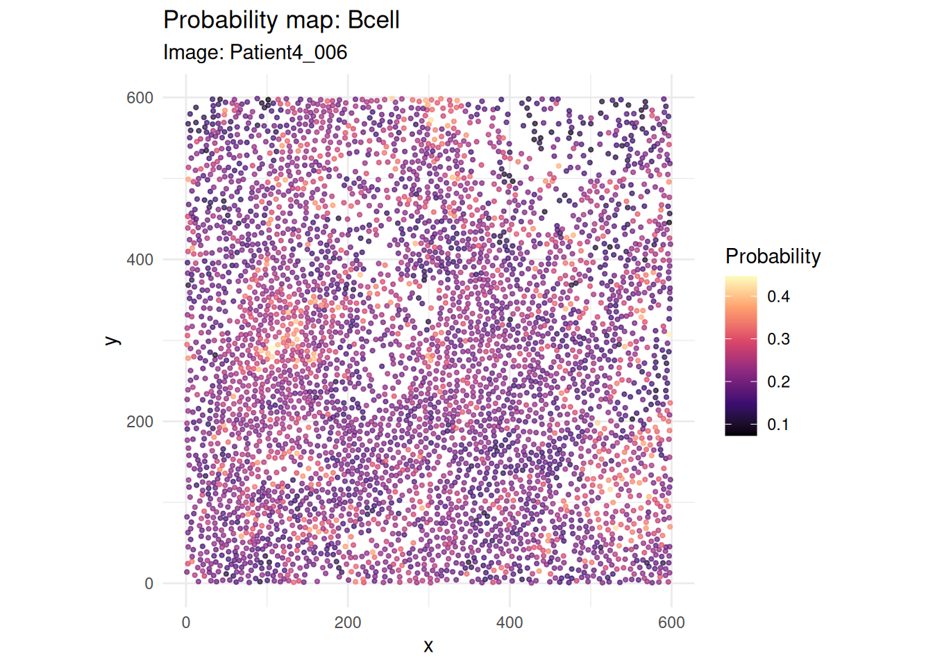
Visualise stored full-workflow probabilities
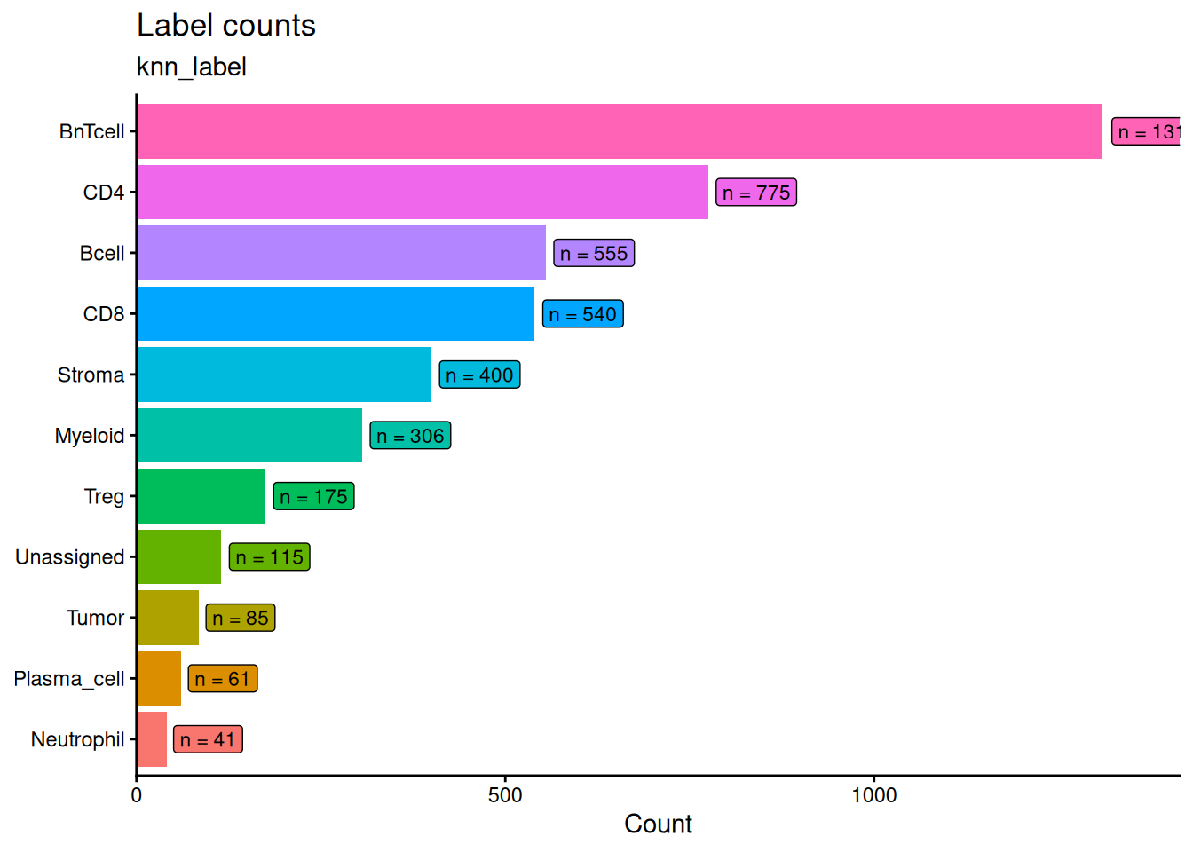
The packaged object contains probabilities from the full ten-lineage demo workflow. These provide a richer example for probability visualisation without rerunning the complete model during vignette construction.
R version 4.6.1 (2026-06-24)
Platform: x86_64-pc-linux-gnu
Running under: Ubuntu 24.04.5 LTS

Matrix products: default
BLAS:   /usr/lib/x86_64-linux-gnu/openblas-pthread/libblas.so.3
LAPACK: /usr/lib/x86_64-linux-gnu/openblas-pthread/libopenblasp-r0.3.26.so;  LAPACK version 3.12.0

locale:
 [1] LC_CTYPE=C.UTF-8       LC_NUMERIC=C           LC_TIME=C.UTF-8
 [4] LC_COLLATE=C.UTF-8     LC_MONETARY=C.UTF-8    LC_MESSAGES=C.UTF-8
 [7] LC_PAPER=C.UTF-8       LC_NAME=C              LC_ADDRESS=C
[10] LC_TELEPHONE=C         LC_MEASUREMENT=C.UTF-8 LC_IDENTIFICATION=C

time zone: UTC
tzcode source: system (glibc)

attached base packages:
[1] stats     graphics  grDevices utils     datasets  methods   base

other attached packages:
[1] cytoGateR_0.99.0

loaded via a namespace (and not attached):
 [1] SummarizedExperiment_1.42.0 gtable_0.3.6
 [3] rjson_0.2.23                xfun_0.61
 [5] ggplot2_4.0.3               ggrepel_0.9.8
 [7] Biobase_2.72.0              lattice_0.22-9
 [9] vctrs_0.7.3                 tools_4.6.1
[11] generics_0.1.4              stats4_4.6.1
[13] proxy_0.4-29                tibble_3.3.1
[15] pkgconfig_2.0.3             Matrix_1.7-5
[17] RColorBrewer_1.1-3          pals_1.10
[19] S7_0.2.2                    S4Vectors_0.50.3
[21] lifecycle_1.0.5             compiler_4.6.1
[23] farver_2.1.2                ggforce_0.5.0
[25] mapproj_1.2.12              Seqinfo_1.2.0
[27] graphlayouts_1.2.5          maps_3.4.3
[29] htmltools_0.5.9             yaml_2.3.12
[31] pillar_1.11.1               tidyr_1.3.2
[33] MASS_7.3-65                 SingleCellExperiment_1.34.0
[35] DelayedArray_0.38.2         cachem_1.1.0
[37] dbscan_1.2.7                magick_2.9.1
[39] viridis_0.6.5               abind_1.4-8
[41] mclust_6.1.3                tidyselect_1.2.1
[43] digest_0.6.39               dplyr_1.2.1
[45] purrr_1.2.2                 labeling_0.4.3
[47] polyclip_1.10-7             fastmap_1.2.0
[49] grid_4.6.1                  colorspace_2.1-4
[51] cli_3.6.6                   SparseArray_1.12.3
[53] magrittr_2.0.5              S4Arrays_1.12.1
[55] dichromat_2.0-1             ggraph_2.2.2
[57] tidygraph_1.3.1             withr_3.0.3
[59] scales_1.4.0                rmarkdown_2.32
[61] XVector_0.52.0              matrixStats_1.5.0
[63] igraph_2.3.4                otel_0.2.0
[65] gridExtra_2.3.1             SpatialExperiment_1.22.0
[67] memoise_2.0.1               evaluate_1.0.5
[69] knitr_1.52                  GenomicRanges_1.64.0
[71] IRanges_2.46.0              viridisLite_0.4.3
[73] rlang_1.3.0                 Rcpp_1.1.2
[75] glue_1.8.1                  tweenr_2.0.3
[77] BiocGenerics_0.58.1         jsonlite_2.0.0
[79] R6_2.6.1                    MatrixGenerics_1.24.0