Overview
Flat classifiers predict among all cell types in a single step. Hierarchical k-nearest-neighbour (kNN) classification instead organizes reference cell types into a tree and predicts one branch at a time. Each internal node separates the cell types on its left branch from those on its right branch. A cell moves recursively through the hierarchy until it reaches a terminal cell type or fails the confidence and agreement requirements.
This vignette demonstrates the complete hierarchical kNN workflow on one complete image from cytoGateR_example.
library(cytoGateR)
data("cytoGateR_example", package = "cytoGateR")

image_ids <- SummarizedExperiment::colData(cytoGateR_example)$image_name
spe <- cytoGateR_example[, image_ids == image_ids[1L]]
spe
class: SpatialExperiment
dim: 40 4363
metadata(0):
assays(1): exprs
rownames(40): MPO H3 ... DNA1 DNA2
rowData names(0):
colnames(4363): 12_1 12_2 ... 12_4371 12_4372
colData names(28): sample_id image_name ... KNN_P_Treg KNN_P_Tumor
reducedDimNames(0):
mainExpName: IMMUcan_2022_CancerExample_v1
altExpNames(0):
spatialCoords names(2) : cell_x cell_y
imgData names(1): sample_id
Prepare reference labels
The packaged core_group column contains high-confidence labels produced by tree gating. Cells outside the high-confidence reference are marked "Unassigned". The hierarchy builders use "Unknown" for cells that should not contribute to the reference, so the labels are harmonized before fitting.
cd <- SummarizedExperiment::colData(spe)
cd$hier_reference_label <- as.character(cd$core_group)
cd$hier_reference_label[cd$hier_reference_label == "Unassigned"] <- "Unknown"
SummarizedExperiment::colData(spe) <- cd

table(SummarizedExperiment::colData(spe)$hier_reference_label)
      Bcell     BnTcell         CD4         CD8     Myeloid  Neutrophil
        236         337         227         206         108          12
Plasma_cell      Stroma        Treg       Tumor     Unknown
         40          71         125          16        2985
Build the lineage hierarchy
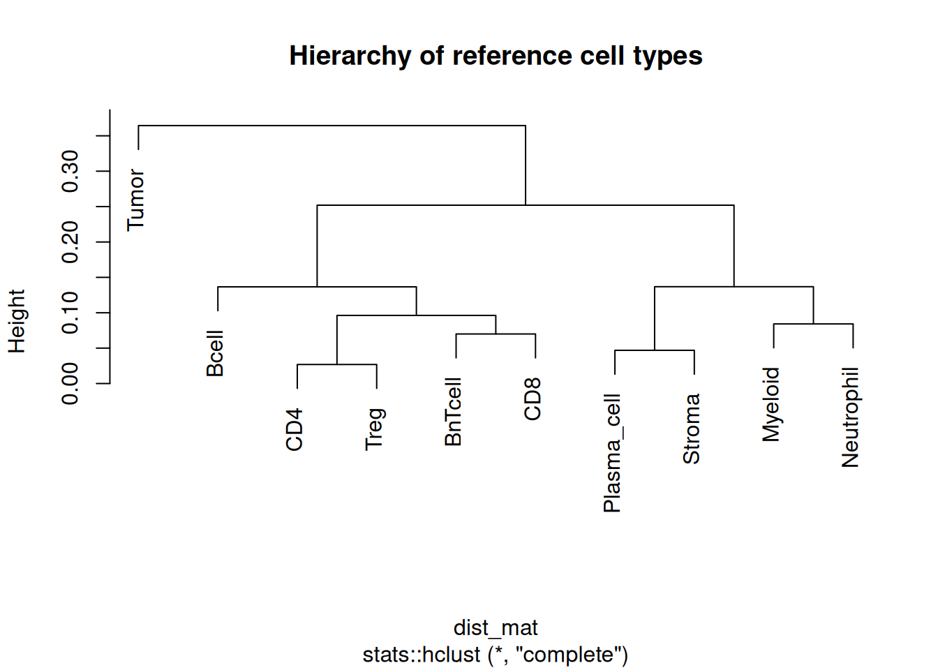
build_lineage_hierarchy() calculates the average marker-expression profile for each reference cell type and hierarchically clusters those profiles.
 [1] "BnTcell"     "CD4"         "Bcell"       "Treg"        "Plasma_cell"
 [6] "Myeloid"     "CD8"         "Stroma"      "Tumor"       "Neutrophil"
plot(hc_tree, main = "Hierarchy of reference cell types")
Build node-specific references
Each internal node receives its own binary training reference. Labels are converted to "Left" and "Right" according to the branches of hc_tree.
Setting top_n = NULL uses all available markers at each node. For larger panels, marker_stats and top_n can be supplied to retain only the most informative markers for each split.
hier_reference <- build_hierarchical_reference(
  spe,
  hc_tree,
  label_col = "hier_reference_label",
  top_n = NULL,
  assay_name = "exprs",
  unknown_label = "Unknown"
)

names(hier_reference)
[1] "Node_1" "Node_2" "Node_3" "Node_4" "Node_5" "Node_6" "Node_7" "Node_8"
[9] "Node_9"
Inspect the root-node reference:
root_name <- paste0("Node_", nrow(hc_tree$merge))
root_reference <- hier_reference[[root_name]]

dim(root_reference$train_data)
table(root_reference$train_labels)
root_reference$left_members
root_reference$right_members
[1] "Bcell"       "CD4"         "Treg"        "BnTcell"     "CD8"
[6] "Plasma_cell" "Stroma"      "Myeloid"     "Neutrophil"
Run recursive hierarchical kNN
At each node, predict_hierarchical_knn_recursive() creates an ensemble of weighted kNN predictions. A prediction is accepted only when both its average probability and ensemble agreement pass their thresholds.
The vignette uses one distance method and one repeat for speed. Production analyses can use multiple distance methods and additional repeats for a more stable ensemble.
set.seed(1)
spe <- predict_hierarchical_knn_recursive(
  spe,
  hier_reference,
  hc_tree,
  assay_name = "exprs",
  threshold = 0.5,
  agreement_threshold = 0.5,
  k = 3,
  repeats = 1,
  dist_methods = "pearson",
  BPPARAM = BiocParallel::SerialParam(),
  out_col = "hier_label",
  chunk_size = 1000,
  unassigned_label = "Unassigned"
)
Inspect hierarchical predictions
      Bcell     BnTcell         CD4         CD8     Myeloid  Neutrophil
        581        1178         882         592         296          22
Plasma_cell      Stroma        Treg       Tumor
        136         425         198          53
The predictions can be compared with labels already stored in the demo object:
             v2
v1            Bcell BnTcell  CD4  CD8 Myeloid Neutrophil Plasma_cell Stroma
  Bcell         479       8   18    8      21          0          16      2
  BnTcell        60    1068  101   64       0          0           0      1
  CD4             4      32  686    7       5          0           5     10
  CD8             0      43   13  457       3          0           7     16
  Myeloid        14       0   13    5     250          3           7     13
  Neutrophil      4       0    3    0       6         18           5      4
  Plasma_cell     1       0    2    3       1          0          48      6
  Stroma          6       0    0    0       2          1          34    356
  Treg            0      11   18    0       0          0           1      2
  Tumor           0       0    0   29       0          0           1      4
  Unassigned     13      16   28   19       8          0          12     11
             v2
v1            Treg Tumor Unassigned
  Bcell          3     0          0
  BnTcell       16     0          0
  CD4           26     0          0
  CD8            0     1          0
  Myeloid        1     0          0
  Neutrophil     0     1          0
  Plasma_cell    0     0          0
  Stroma         1     0          0
  Treg         143     0          0
  Tumor          0    51          0
  Unassigned     8     0          0
         label match_n union_n agreement
1        Bcell     479     657 0.7290715
2      BnTcell    1068    1420 0.7521127
3          CD4     686     971 0.7064882
4          CD8     457     675 0.6770370
5      Myeloid     250     352 0.7102273
6   Neutrophil      18      45 0.4000000
7  Plasma_cell      48     149 0.3221477
8       Stroma     356     469 0.7590618
9         Treg     143     230 0.6217391
10       Tumor      51      87 0.5862069
11  Unassigned       0     115 0.0000000
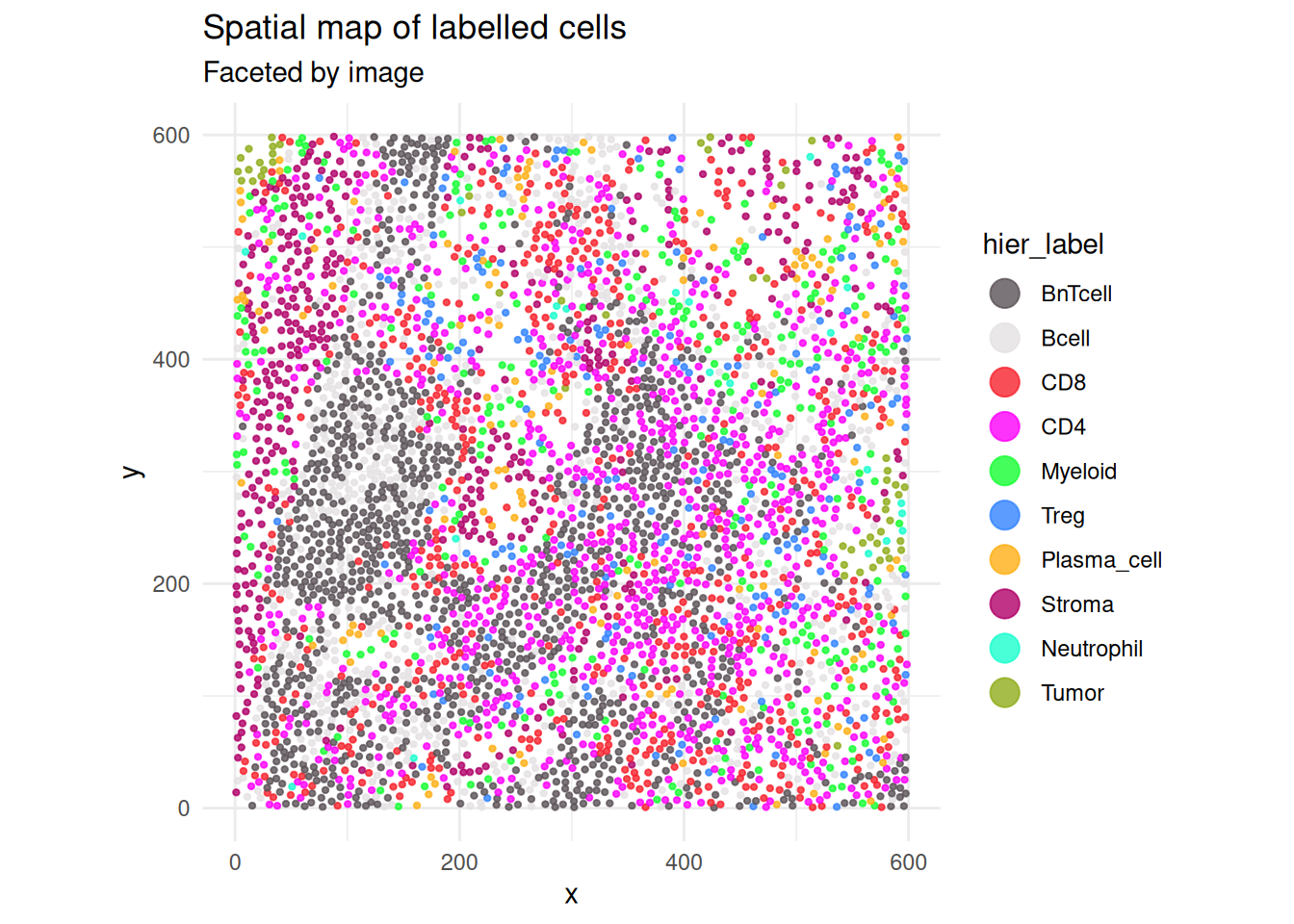
Finally, display the hierarchical predictions in spatial coordinates:
Production settings
A larger ensemble can combine correlation- and angle-based similarity measures:
R version 4.6.1 (2026-06-24)
Platform: x86_64-pc-linux-gnu
Running under: Ubuntu 24.04.5 LTS

Matrix products: default
BLAS:   /usr/lib/x86_64-linux-gnu/openblas-pthread/libblas.so.3
LAPACK: /usr/lib/x86_64-linux-gnu/openblas-pthread/libopenblasp-r0.3.26.so;  LAPACK version 3.12.0

locale:
 [1] LC_CTYPE=C.UTF-8       LC_NUMERIC=C           LC_TIME=C.UTF-8
 [4] LC_COLLATE=C.UTF-8     LC_MONETARY=C.UTF-8    LC_MESSAGES=C.UTF-8
 [7] LC_PAPER=C.UTF-8       LC_NAME=C              LC_ADDRESS=C
[10] LC_TELEPHONE=C         LC_MEASUREMENT=C.UTF-8 LC_IDENTIFICATION=C

time zone: UTC
tzcode source: system (glibc)

attached base packages:
[1] stats     graphics  grDevices utils     datasets  methods   base

other attached packages:
[1] cytoGateR_0.99.0

loaded via a namespace (and not attached):
 [1] SummarizedExperiment_1.42.0 gtable_0.3.6
 [3] rjson_0.2.23                xfun_0.61
 [5] ggplot2_4.0.3               ggrepel_0.9.8
 [7] Biobase_2.72.0              lattice_0.22-9
 [9] vctrs_0.7.3                 tools_4.6.1
[11] generics_0.1.4              parallel_4.6.1
[13] stats4_4.6.1                proxy_0.4-29
[15] tibble_3.3.1                pkgconfig_2.0.3
[17] Matrix_1.7-5                RColorBrewer_1.1-3
[19] pals_1.10                   S7_0.2.2
[21] S4Vectors_0.50.3            lifecycle_1.0.5
[23] compiler_4.6.1              farver_2.1.2
[25] ggforce_0.5.0               mapproj_1.2.12
[27] codetools_0.2-20            Seqinfo_1.2.0
[29] graphlayouts_1.2.5          maps_3.4.3
[31] htmltools_0.5.9             yaml_2.3.12
[33] pillar_1.11.1               tidyr_1.3.2
[35] MASS_7.3-65                 BiocParallel_1.46.0
[37] SingleCellExperiment_1.34.0 DelayedArray_0.38.2
[39] cachem_1.1.0                dbscan_1.2.7
[41] magick_2.9.1                viridis_0.6.5
[43] abind_1.4-8                 mclust_6.1.3
[45] tidyselect_1.2.1            digest_0.6.39
[47] dplyr_1.2.1                 purrr_1.2.2
[49] labeling_0.4.3              polyclip_1.10-7
[51] fastmap_1.2.0               grid_4.6.1
[53] colorspace_2.1-4            cli_3.6.6
[55] SparseArray_1.12.3          magrittr_2.0.5
[57] S4Arrays_1.12.1             dichromat_2.0-1
[59] ggraph_2.2.2                tidygraph_1.3.1
[61] withr_3.0.3                 scales_1.4.0
[63] rmarkdown_2.32              XVector_0.52.0
[65] matrixStats_1.5.0           igraph_2.3.4
[67] otel_0.2.0                  gridExtra_2.3.1
[69] SpatialExperiment_1.22.0    memoise_2.0.1
[71] evaluate_1.0.5              knitr_1.52
[73] GenomicRanges_1.64.0        IRanges_2.46.0
[75] viridisLite_0.4.3           rlang_1.3.0
[77] Rcpp_1.1.2                  glue_1.8.1
[79] tweenr_2.0.3                BiocGenerics_0.58.1
[81] jsonlite_2.0.0              R6_2.6.1
[83] MatrixGenerics_1.24.0