4 Cell segmentation and pre-processing
The typical first step in analysing spatial data is cell segmentation, which involves identifying and isolating individual cells in each image. This defines the basic units (cells) on which most downstream omics analysis is performed.
There are multiple approaches to cell segmentation. One approach involves segmenting the nuclei using intensity-based thresholding of a nuclear marker (such as DAPI or Histone H3), followed by watershedding to separate touching cells. The segmented nuclei are then expanded by a fixed or adaptive radius to approximate the full cell body. While this method is straightforward and widely used, especially when only nuclear staining is available, it assumes uniform cell size and shape, which may not hold in heterogeneous tissues.
When membrane or cytoplasmic markers are present, they can be used to directly segment the full cell body. This provides a more accurate representation of cell shape and size, particularly in tissues where cells are irregular or closely packed.
The choice of segmentation strategy depends on tissue structure, cell density, imaging resolution, and the biological questions at hand. In densely packed tissues such as epithelium or tumour microenvironments, clear boundary definition is challenging, and over-segmentation is often preferred to minimise signal spillover. In contrast, broader segmentation may be more appropriate in sparse tissues to capture full cell morphology. This trade-off is especially important when analysing membrane or cytoplasmic markers, where accurate capture of the cell body is essential to avoid background contamination or misattribution of signal.
To balance marker quantification and minimise spillover, we recommend nuclear segmentation followed by fixed-radius dilation to approximate the cytoplasm. In this section, we demonstrate how the simpleSeg package implements this approach, and outline additional options for users requiring greater flexibility.
The code below automatically detects the number of available CPU cores on your system and configures parallel processing accordingly. If you’re on a Windows machine, it uses a socket-based backend (SnowParam), while Unix-based systems (macOS/Linux) use a fork-based backend (MulticoreParam).
If only one core is available or parallel execution is disabled, it defaults to serial processing. We recommend using at least 2 cores as parts of the workflow can be computationally intensive. If you do not wish to use multiple cores, you can set use_mc = FALSE.
# set parameters
set.seed(51773)

# whether to use multiple cores (recommended)
use_mc = TRUE
is_windows = .Platform$OS.type == "windows"

if (use_mc) {
  nCores = max(ceiling(parallel::detectCores() / 2), 1)

  if (nCores == 1) {
    BPPARAM = BiocParallel::SerialParam()
  } else if (is_windows) {
    BPPARAM = BiocParallel::SnowParam(workers = nCores, type = "SOCK")
  } else {
    BPPARAM = BiocParallel::MulticoreParam(workers = nCores)
  }
} else {
  BPPARAM = BiocParallel::SerialParam()
}

theme_set(theme_classic())
4.1 Reading in data with cytomapper
We will be using the Ferguson 2022 dataset to demonstrate how to perform pre-processing and cell segmentation. This dataset can be accessed through the SpatialDatasets package and is available in the form of single-channel TIFF images. In single-channel images, each pixel represents intensity values for a single marker. The loadImages function from the cytomapper package can be used to load all the TIFF images into a CytoImageList object. We then store the images as an h5 file on-disk in a temporary directory using the h5FilesPath = HDF5Array::getHDF5DumpDir() parameter.
We will also assign the metadata columns of the CytoImageList object using the mcols function.
pathToZip <- SpatialDatasets::Ferguson_Images()
pathToImages <- "data/processing/images"
unzip(pathToZip, exdir = "data/processing/images")

# store images in a CytoImageList on_disk as h5 files to save memory
images <- cytomapper::loadImages(
  pathToImages,
  single_channel = TRUE,
  on_disk = TRUE,
  h5FilesPath = HDF5Array::getHDF5DumpDir(),
  BPPARAM = BPPARAM
)

# assign metadata columns
mcols(images) <- S4Vectors::DataFrame(imageID = names(images))When reading the image channels directly from the names of the TIFF images, they will often need to be cleaned for ease of downstream processing. The channel names can be accessed from the CytoImageList object using the channelNames function.
channelNames(images) <- channelNames(images) |>
                          # remove preceding letters
                          sub(pattern = ".*_", replacement = "", x = _) |>
                          # remove the .ome
                          sub(pattern = ".ome", replacement = "", x = _)
Similarly, the image names will be taken from the folder name containing the individual TIFF images for each channel. These will often also need to be cleaned.
4.2 Cell segmentation with simpleSeg
For the sake of simplicity and efficiency, we will be subsetting the images down to 10 images.
images <- images[1:10]Next, we can perform our segmentation. The simpleSeg package on Bioconductor provides functionality for user friendly, watershed based segmentation on multiplexed cellular images based on the intensity of user-specified marker channels. The main function, simpleSeg, can be used to perform a simple cell segmentation process that traces out the nuclei using a specified channel.
In the particular example below, we have asked simpleSeg to do the following:
-
nucleus = c("HH3"): trace out the nuclei signal in the images using the HH3 channel. -
pca = TRUE: segment out the nuclei mask using principal component analysis of all channels and using the principal components most aligned with the nuclei channel (in this case, HH3). -
cellBody = "dilate": use a dilation strategy of segmentation, expanding out from the nucleus by a specifieddiscSize. In this case,discSize = 3, which means simpleSeg dilates out from the nucleus by 3 pixels. -
sizeSelection = 20: ensure that only cells with a size greater than 20 pixels will be used. -
transform = "sqrt": perform square root transformation on each of the channels prior to segmentation. -
tissue = c("panCK", "CD45", "HH3"): use the specified tissue mask to filter out all background noise outside the tissue mask. This allows us to ignore background noise which happens outside of the tumour core.
There are many other parameters that can be specified in simpleSeg (smooth, watershed, tolerance, and ext), and we encourage the user to select the parameters which best suit their biological context.
masks <- simpleSeg(images,
                   nucleus = c("HH3"),
                   pca = TRUE,
                   cellBody = "dilate",
                   discSize = 3,
                   sizeSelection = 20,
                   transform = "sqrt",
                   tissue = c("panCK", "CD45", "HH3"),
cores = nCores)4.2.1 Visualise separation
We can examine the performance of the cell segmentation using the display and colorLabels functions from the EBImage package. If used in an interactive session, display allows you to zoom in and out of the image. In the image below, each distinct colour represents an individual segmented nucleus.
# display image F3
EBImage::display(colorLabels(masks[[1]]))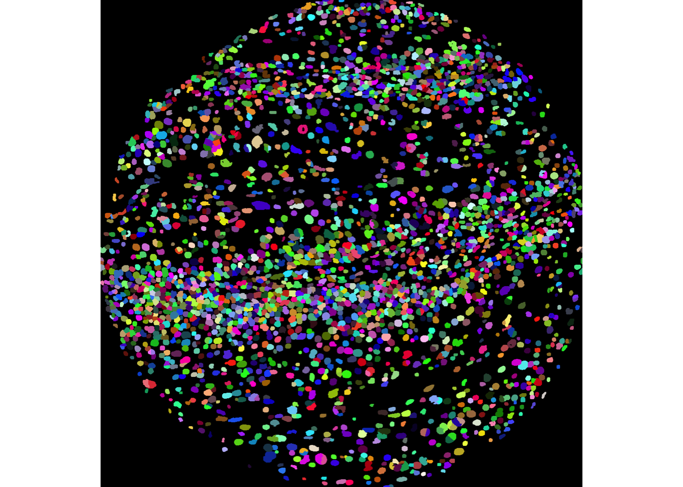
4.2.2 Visualise outlines
To assess segmentation accuracy, we can overlay the nuclei masks onto the corresponding nuclear intensity channel. Ideally, the mask outlines (shown in white in the image below) should closely align with the boundaries of the nuclear signal (visualised in blue), indicating that the segmentation correctly captures the extent of each nucleus. To do this, we can use the plotPixels function from the cytomapper package.
plotPixels(image = images["F3"],
           mask = masks["F3"],
           img_id = "imageID",
           colour_by = c("HH3"),
           display = "single",
           colour = list(HH3 = c("black","blue")),
           legend = NULL,
           bcg = list(
             HH3 = c(1, 1, 2)
           ))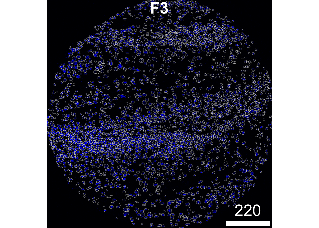
Now is a good time to check whether we are over- or under-segmenting.
Over-segmentation happens when one cell or nucleus gets split into multiple smaller segments. This can lead to inflated cell counts and fragmented masks, which might skew your downstream analyses. Visually, you’ll see lots of small, irregular segments clustered where there should be just one cell.
Under-segmentation is the opposite — when two or more neighboring cells or nuclei are merged into a single segment. This causes under-counting and can hide important biological differences. You might notice large, oddly shaped masks covering what should be separate cells.
If you spot over- or under-segmentation in your images, adjusting the discSize parameter in the simpleSeg function can help. This controls the size of the dilation applied after nuclei segmentation, and tuning it can improve how well the masks approximate the actual cell boundaries.
It’s also useful to look at multiple markers at once — not just the nuclear marker (HH3) — to get a fuller picture of how well the segmentation masks fit the cells in your tissue. Below, we’ve visualised the same image with additional markers: HH3, CD31, FX111A.
plotPixels(image = images["F3"],
           mask = masks["F3"],
           img_id = "imageID",
           colour_by = c("HH3", "CD31", "FX111A"),
           display = "single",
           colour = list(HH3 = c("black","blue"),
                         CD31 = c("black", "red"),
                         FX111A = c("black", "green")),
           legend = NULL,
           bcg = list(
             HH3 = c(1, 1, 2),
             CD31 = c(0, 1, 2),
             FX111A = c(0, 1, 1.5)
           ))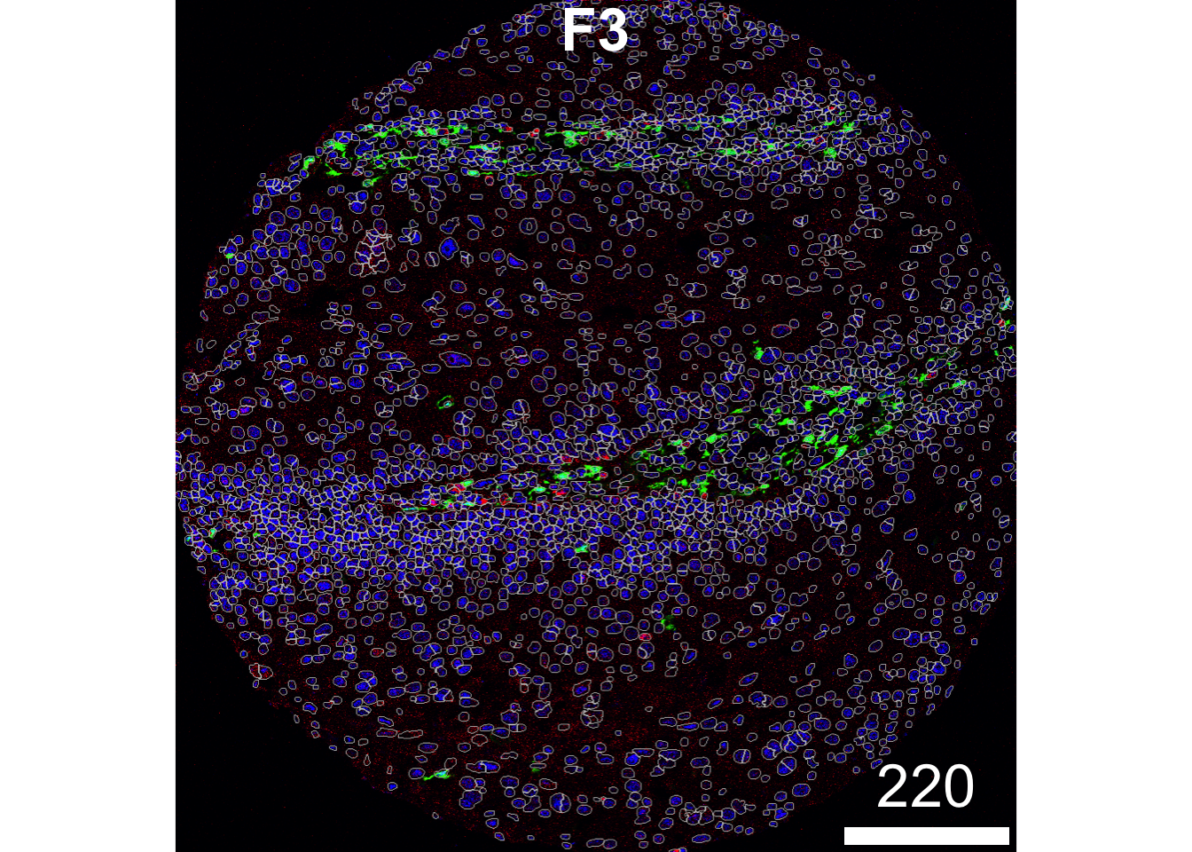
In the image above, our segmentation does a good job capturing the CD31 signal (red), but is less accurate for the FX111A signal (green). You can see areas where the FX111A signal extends beyond the boundaries of our segmentation masks. There are clear regions where the FX111A marker spills over the boundaries of our segmentation. We could rectify this by increasing the discSize to capture more of the cell body.
However, it’s important to consider lateral spillover — a common challenge in spatial analysis. Lateral spillover occurs when signal from one cell spreads into neighboring cells, causing the marker intensity to be incorrectly assigned to adjacent cells. This can happen due to the natural diffusion of cytoplasmic or membrane-bound proteins, limitations in segmentation accuracy, or imaging resolution.
Balancing the dilation size to capture the full cell body while minimising lateral spillover is therefore crucial. Overly large segmentation masks may increase spillover, while masks that are too small risk missing important cellular signals.
What to look for and change to obtain an ideal segmentation
- Does the segmentation capture the full nucleus? If not, perhaps you need to try a different transformation to improve the thresholding of the nuclei marker. You could also try using
pca = TRUEwhich will borrow information across the markers to help find the nuclei. - How much of the cell body is the segmentation missing? Try increasing the dilation around the nucleus by setting
discSize = 7. - Are the segmentations capturing neighbouring cells? Try decreasing the dilation to limit lateral spillover of marker signal by setting
discSize = 2.
In particular, the cellBody and watershed parameters can strongly influence the way cells are segmented using simpleSeg. We have provided further details on how the user may specify cell body identification and watershedding in the tables below.
As simpleSeg is a nuclei-based dilation method, it suffers from tissues where cells might be multi-nucleated, or where cells have non-circular or elliptical morphologies. For tissues where you might expect these cells, it may be preferable to choose a different segmentation method.
4.2.2.1 cellBody Parameters
| Method | Description |
|---|---|
| “distance” | Performs watershedding on a distance map of the thresholded nuclei signal. With a pixels distance being defined as the distance from the closest background signal. |
| “intensity” | Performs watershedding using the intensity of the nuclei marker. |
| “combine” | Combines the previous two methods by multiplying the distance map by the nuclei marker intensity. |
4.2.2.2 watershed Parameters
| Method | Description |
|---|---|
| “dilation” | Dilates the nuclei by an amount defined by the user. The size of the dilatation in pixels may be specified with the discDize argument. |
| “discModel” | Uses all the markers to predict the presence of dilated ‘discs’ around the nuclei. The model therefore learns which markers are typically present in the cell cytoplasm and generates a mask based on this. |
| “marker” | The user may specify one or multiple dedicated cytoplasm markers to predict the cytoplasm. This can be done using cellBody = "marker name"/"index" |
| “None” | The nuclei mask is returned directly. |
4.3 Summarise cell features
In the Bioconductor ecosystem, the SingleCellExperiment and SpatialExperiment classes are widely used data structures for storing single-cell and spatially resolved data, along with associated metadata. We recommend using these formats for downstream analysis in R, as they are well-supported across many packages.
To extract per-cell measurements from segmentation masks, we can use the measureObjects function from the cytomapper package. This calculates the average intensity of each channel within each cell, along with various morphological features. By default, measureObjects returns a SingleCellExperiment, where channel intensities are stored in the counts assay, and spatial coordinates are included in colData under the m.cx and m.cy columns.
Alternatively, setting return_as = "spe" will return a SpatialExperiment object instead. In this format, spatial coordinates are stored in the spatialCoords slot, which simplifies integration with spatial analysis workflows and plotting functions. For this demonstration, we’ll use the SpatialExperiment format.
# summarise the expression of each marker in each cell
cells <- cytomapper::measureObjects(masks,
                                    images,
                                    img_id = "imageID",
                                    return_as = "spe",
                                    BPPARAM = BPPARAM)

spatialCoordsNames(cells) <- c("x", "y")

cells
class: SpatialExperiment
dim: 36 37979
metadata(0):
assays(1): counts
rownames(36): panCK CD20 ... DNA1 DNA2
rowData names(0):
colnames: NULL
colData names(8): imageID object_id ... sample_id objectNum
reducedDimNames(0):
mainExpName: NULL
altExpNames(0):
spatialCoords names(2) : x y
imgData names(1): sample_idIn the next section, we’ll look at performing quality control, data transformation, and normalisation to account for technical variation and prepare the data for analysis.
4.4 sessionInfo
R version 4.5.0 (2025-04-11)
Platform: aarch64-apple-darwin20
Running under: macOS Sonoma 14.4.1

Matrix products: default
BLAS:   /Library/Frameworks/R.framework/Versions/4.5-arm64/Resources/lib/libRblas.0.dylib
LAPACK: /Library/Frameworks/R.framework/Versions/4.5-arm64/Resources/lib/libRlapack.dylib;  LAPACK version 3.12.1

locale:
[1] en_US.UTF-8/en_US.UTF-8/en_US.UTF-8/C/en_US.UTF-8/en_US.UTF-8

time zone: Australia/Sydney
tzcode source: internal

attached base packages:
[1] stats4    stats     graphics  grDevices utils     datasets  methods
[8] base

other attached packages:
 [1] SpatialDatasets_1.6.3       SpatialExperiment_1.18.1
 [3] ExperimentHub_2.16.0        AnnotationHub_3.16.0
 [5] BiocFileCache_2.16.0        dbplyr_2.5.0
 [7] simpleSeg_1.9.2             ggplot2_3.5.2
 [9] cytomapper_1.20.0           SingleCellExperiment_1.30.1
[11] SummarizedExperiment_1.38.1 Biobase_2.68.0
[13] GenomicRanges_1.60.0        GenomeInfoDb_1.44.0
[15] IRanges_2.42.0              S4Vectors_0.46.0
[17] BiocGenerics_0.54.0         generics_0.1.4
[19] MatrixGenerics_1.20.0       matrixStats_1.5.0
[21] EBImage_4.50.0

loaded via a namespace (and not attached):
  [1] DBI_1.2.3               bitops_1.0-9            deldir_2.0-4
  [4] gridExtra_2.3           rlang_1.1.6             magrittr_2.0.3
  [7] svgPanZoom_0.3.4        shinydashboard_0.7.3    compiler_4.5.0
 [10] RSQLite_2.3.11          spatstat.geom_3.4-1     png_0.1-8
 [13] systemfonts_1.2.3       fftwtools_0.9-11        vctrs_0.6.5
 [16] pkgconfig_2.0.3         crayon_1.5.3            fastmap_1.2.0
 [19] magick_2.8.5            XVector_0.48.0          promises_1.3.2
 [22] rmarkdown_2.29          UCSC.utils_1.4.0        ggbeeswarm_0.7.2
 [25] purrr_1.0.4             bit_4.6.0               xfun_0.52
 [28] cachem_1.1.0            jsonlite_2.0.0          blob_1.2.4
 [31] later_1.4.2             rhdf5filters_1.20.0     DelayedArray_0.34.1
 [34] spatstat.utils_3.1-4    Rhdf5lib_1.30.0         BiocParallel_1.42.0
 [37] jpeg_0.1-11             tiff_0.1-12             terra_1.8-50
 [40] parallel_4.5.0          R6_2.6.1                RColorBrewer_1.1-3
 [43] spatstat.data_3.1-6     spatstat.univar_3.1-3   Rcpp_1.0.14
 [46] knitr_1.50              httpuv_1.6.16           Matrix_1.7-3
 [49] nnls_1.6                tidyselect_1.2.1        yaml_2.3.10
 [52] rstudioapi_0.17.1       dichromat_2.0-0.1       abind_1.4-8
 [55] viridis_0.6.5           codetools_0.2-20        curl_6.2.3
 [58] lattice_0.22-6          tibble_3.2.1            KEGGREST_1.48.0
 [61] shiny_1.10.0            withr_3.0.2             evaluate_1.0.3
 [64] polyclip_1.10-7         Biostrings_2.76.0       filelock_1.0.3
 [67] BiocManager_1.30.25     pillar_1.10.2           sp_2.2-0
 [70] RCurl_1.98-1.17         BiocVersion_3.21.1      scales_1.4.0
 [73] xtable_1.8-4            glue_1.8.0              tools_4.5.0
 [76] locfit_1.5-9.12         rhdf5_2.52.0            grid_4.5.0
 [79] AnnotationDbi_1.70.0    colorspace_2.1-1        GenomeInfoDbData_1.2.14
 [82] raster_3.6-32           beeswarm_0.4.0          HDF5Array_1.36.0
 [85] vipor_0.4.7             cli_3.6.5               rappdirs_0.3.3
 [88] textshaping_1.0.1       S4Arrays_1.8.0          viridisLite_0.4.2
 [91] svglite_2.2.1           dplyr_1.1.4             gtable_0.3.6
 [94] digest_0.6.37           SparseArray_1.8.0       rjson_0.2.23
 [97] htmlwidgets_1.6.4       farver_2.1.2            memoise_2.0.1
[100] htmltools_0.5.8.1       lifecycle_1.0.4         h5mread_1.0.1
[103] httr_1.4.7              mime_0.13               bit64_4.6.0-1