9 Identifying spatial domains with unsupervised clustering
Beyond pairwise spatial relationships between cell types, imaging datasets reveal richer layers of tissue organisation through concepts like niches, neighborhoods, microenvironments, and spatial domains. Niches typically describe the immediate surroundings of a specific cell, while spatial domains represent larger tissue compartments formed by coordinated cell arrangements. These frameworks help us understand how tissue architecture varies across conditions or patient groups.
The interpretation of spatial domains is highly context-dependent. In cancer research, domain analysis might highlight the distribution of tumor and immune compartments or reveal how domain composition correlates with disease progression. In metabolic diseases like diabetes, domains such as pancreatic islets serve as key regions for studying changes in marker expression or immune infiltration.

One effective approach to identify spatial domains involves clustering cells based on their local spatial association patterns, as implemented in the lisaClust package. This method groups tissue regions with similar spatial signatures, uncovering emergent domains within complex tissue landscapes. Selecting the appropriate number of clusters and interpreting them based on cell type composition and density remains a key challenge. While statistical metrics like the Gap statistic or Silhouette score can help guide cluster selection, biological insight is crucial to distinguish meaningful structural patterns from noise.
In this section, we demonstrate how to use lisaClust to identify spatial domains and examine their relevance to clinical outcomes.
# set parameters
set.seed(51773)

# whether to use multiple cores (recommended)
use_mc = TRUE
is_windows = .Platform$OS.type == "windows"

if (use_mc) {
  nCores = max(ceiling(parallel::detectCores() / 2), 1)

  if (nCores == 1) {
    BPPARAM = BiocParallel::SerialParam()
  } else if (is_windows) {
    BPPARAM = BiocParallel::SnowParam(workers = nCores, type = "SOCK")
  } else {
    BPPARAM = BiocParallel::MulticoreParam(workers = nCores)
  }
} else {
  BPPARAM = BiocParallel::SerialParam()
}

theme_set(theme_classic())
9.1 lisaClust
lisaClust is a method developed to identify and characterize tissue microenvironments from highly multiplexed imaging data by analyzing how different types of cells are arranged in space. It starts by treating each cell as a point on a 2D map, with each point labeled by its cell type. For every individual cell, lisaClust calculates how strongly it is surrounded by other specific cell types—more or less than would be expected by chance—using spatial statistics called the K-function or L-function. These calculations, called local indicators of spatial association (LISAs), capture detailed information about local cell–cell interactions across the tissue.

lisaClust then uses these cell-level spatial profiles to group cells into clusters using standard clustering algorithms like k-means. Each cluster represents a tissue region, or microenvironment, where certain combinations of cell types tend to co-occur in space. This approach allows researchers to move beyond simple pairwise analyses and uncover more complex patterns of organization, like immune niches or tumour–stroma boundaries, that reflect how cells interact within the broader tissue context.
9.1.1 Case study: Keren
We will start by reading in the Keren 2018 dataset from the SpatialDatasets package as a SingleCellExperiment object. Here the data is in a format consistent with that outputted by CellProfiler.
kerenSPE <- SpatialDatasets::spe_Keren_2018()see ?SpatialDatasets and browseVignettes('SpatialDatasets') for documentationloading from cache9.1.1.1 Generate LISA curves
For the purpose of this demonstration, we will be using only images 5 and 6 of the dataset.
This data comes with pre-annotated cell types, so we can move directly to performing k-means clustering on the local indicators of spatial association (LISA) functions using the lisaClust function. The image ID, cell type column, and spatial coordinates can be specified using the imageID, cellType, and spatialCoords arguments respectively. We will identify 5 regions of co-localisation by setting k = 5.
kerenSPE <- lisaClust(kerenSPE,
                      k = 5)
These regions are stored in colData and can be extracted.
DataFrame with 10 rows and 2 columns
          imageID      region
      <character> <character>
21154           5    region_4
21155           5    region_4
21156           5    region_4
21157           5    region_2
21158           5    region_2
21159           5    region_2
21160           5    region_5
21161           5    region_2
21162           5    region_2
21163           5    region_2
9.1.1.2 Examine cell type enrichment
lisaClust also provides a convenient function, regionMap, for examining which cell types are located in which regions. In this example, we use this to check which cell types appear more frequently in each region than expected by chance.
regionMap(kerenSPE,
  type = "bubble")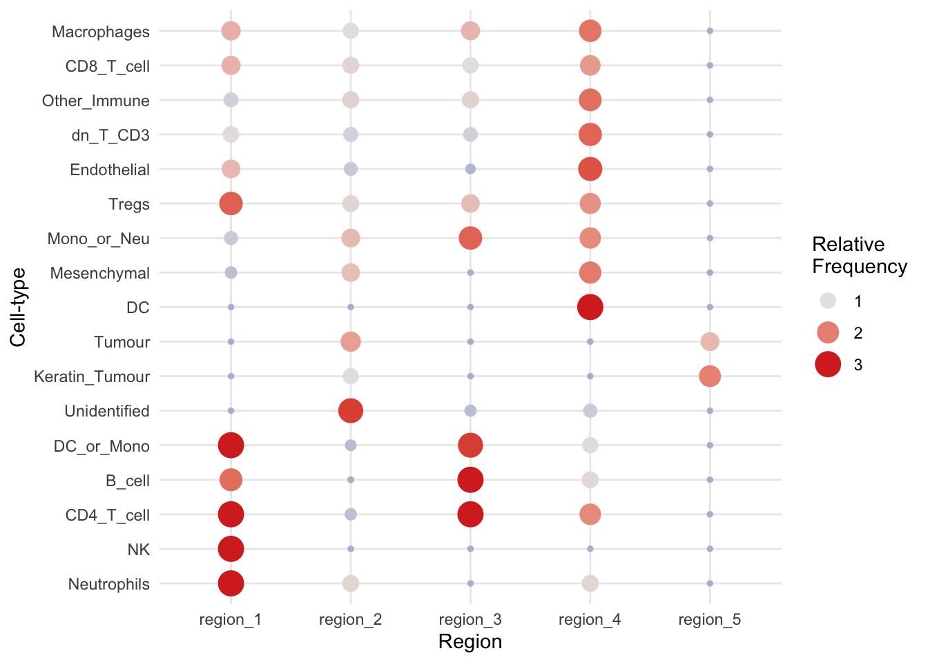
Above, we can see that tumour cells are concentrated in region 5, and immune cells are concentrated in region 1 and 4. We can further segregate these cells by increasing the number of clusters, i.e., increasing the parameter k = in the lisaClust function.
In addition to choosing an appropriate number of clusters, it is equally important to select a biologically meaningful radius over which spatial associations are calculated. The radius determines the scale at which local neighbourhoods are defined—essentially setting the window for detecting co-localisation patterns. A small radius focuses on immediate cellular environments and short-range interactions, making it ideal for identifying tightly organised niches or direct cell–cell contact. In contrast, a larger radius captures broader patterns, such as tissue compartmentalisation or gradient-based organisation. The optimal radius should reflect the biological scale of interest, such as known signalling distances or histological structures, and it can be helpful to explore multiple values to understand how spatial organisation changes across scales.
How do we choose an appropriate value for k?
The choice of
kdepends largely on the biological question being asked. For instance, if we are interested in understanding the interactions between immune cells in a tumor microenvironment, the number of clusters should reflect the known biological subtypes of immune cells, such as T cells, B cells, macrophages, etc. In this case, a larger value ofkmay be needed to capture the diversity within these immune cell populations.On the other hand, if the focus is on interactions between immune cells and tumor cells, we might choose a smaller value of
kto group immune cells into broader categories.Additionally, methods like the Gap statistic, Jump statistic, or Silhouette score could be employed to determine an optimal value of
k.
9.1.1.3 Plot identified regions
We can use the hatchingPlot function to visualise all 5 regions and 17 cell types simultaneously for a specific image or set of images. The output is a ggplot object where the regions are marked by different hatching patterns. The nbp argument can be used to tune the granularity of the grid used for defining regions.
hatchingPlot(kerenSPE, useImages = 5, nbp = 300)Concave windows are temperamental. Try choosing values of window.length > and < 1 if you have problems.Warning in split.default(x = seq_len(nrow(x)), f = f, drop = drop, ...): data
length is not a multiple of split variable
Warning in split.default(x = seq_len(nrow(x)), f = f, drop = drop, ...): data
length is not a multiple of split variable
In accordance with the regionMap output, we can see that region 5 is mostly made up of tumour cells, and region 2 and 4 both contain our immune cell populations.
How could results from lisaClust be used in conjunction with results from spicyR?
lisaClust provides a high-resolution view of the tissue architecture, while spicyR can quantify how these spatial relationships or features contribute to clinical outcomes. spicyR’s L-function metric can be used to determine the degree of localisation or dispersion between different spatial domains. For instance, we can look at co-localisation between region 5 (our tumour cells) and regions 2 or 4 (our immune cells).
9.2 sessionInfo
R version 4.5.0 (2025-04-11)
Platform: aarch64-apple-darwin20
Running under: macOS Sonoma 14.4.1

Matrix products: default
BLAS:   /Library/Frameworks/R.framework/Versions/4.5-arm64/Resources/lib/libRblas.0.dylib
LAPACK: /Library/Frameworks/R.framework/Versions/4.5-arm64/Resources/lib/libRlapack.dylib;  LAPACK version 3.12.1

locale:
[1] en_US.UTF-8/en_US.UTF-8/en_US.UTF-8/C/en_US.UTF-8/en_US.UTF-8

time zone: Australia/Sydney
tzcode source: internal

attached base packages:
[1] stats4    stats     graphics  grDevices utils     datasets  methods
[8] base

other attached packages:
 [1] SpatialDatasets_1.6.3       SpatialExperiment_1.18.1
 [3] ExperimentHub_2.16.0        AnnotationHub_3.16.0
 [5] BiocFileCache_2.16.0        dbplyr_2.5.0
 [7] SingleCellExperiment_1.30.1 SummarizedExperiment_1.38.1
 [9] Biobase_2.68.0              GenomicRanges_1.60.0
[11] GenomeInfoDb_1.44.0         IRanges_2.42.0
[13] S4Vectors_0.46.0            BiocGenerics_0.54.0
[15] generics_0.1.4              MatrixGenerics_1.20.0
[17] matrixStats_1.5.0           ggplot2_3.5.2
[19] spicyR_1.20.1               lisaClust_1.16.0

loaded via a namespace (and not attached):
  [1] later_1.4.2                 splines_4.5.0
  [3] bitops_1.0-9                filelock_1.0.3
  [5] svgPanZoom_0.3.4            tibble_3.2.1
  [7] polyclip_1.10-7             lifecycle_1.0.4
  [9] Rdpack_2.6.4                rstatix_0.7.2
 [11] lattice_0.22-6              MASS_7.3-65
 [13] MultiAssayExperiment_1.34.0 backports_1.5.0
 [15] magrittr_2.0.3              rmarkdown_2.29
 [17] yaml_2.3.10                 httpuv_1.6.16
 [19] doRNG_1.8.6.2               ClassifyR_3.12.0
 [21] sp_2.2-0                    dcanr_1.24.0
 [23] spatstat.sparse_3.1-0       DBI_1.2.3
 [25] minqa_1.2.8                 RColorBrewer_1.1-3
 [27] abind_1.4-8                 purrr_1.0.4
 [29] RCurl_1.98-1.17             tweenr_2.0.3
 [31] rappdirs_0.3.3              GenomeInfoDbData_1.2.14
 [33] spatstat.utils_3.1-4        terra_1.8-50
 [35] pheatmap_1.0.12             goftest_1.2-3
 [37] simpleSeg_1.9.2             spatstat.random_3.4-1
 [39] svglite_2.2.1               codetools_0.2-20
 [41] DelayedArray_0.34.1         ggforce_0.4.2
 [43] tidyselect_1.2.1            raster_3.6-32
 [45] UCSC.utils_1.4.0            farver_2.1.2
 [47] viridis_0.6.5               lme4_1.1-37
 [49] spatstat.explore_3.4-3      jsonlite_2.0.0
 [51] Formula_1.2-5               survival_3.8-3
 [53] iterators_1.0.14            systemfonts_1.2.3
 [55] foreach_1.5.2               tools_4.5.0
 [57] ggnewscale_0.5.1            Rcpp_1.0.14
 [59] glue_1.8.0                  gridExtra_2.3
 [61] SparseArray_1.8.0           BiocBaseUtils_1.10.0
 [63] xfun_0.52                   mgcv_1.9-3
 [65] ggthemes_5.1.0              EBImage_4.50.0
 [67] HDF5Array_1.36.0            dplyr_1.1.4
 [69] shinydashboard_0.7.3        scam_1.2-19
 [71] withr_3.0.2                 numDeriv_2016.8-1.1
 [73] BiocManager_1.30.25         fastmap_1.2.0
 [75] ggh4x_0.3.0                 rhdf5filters_1.20.0
 [77] boot_1.3-31                 digest_0.6.37
 [79] R6_2.6.1                    mime_0.13
 [81] textshaping_1.0.1           colorspace_2.1-1
 [83] tensor_1.5                  jpeg_0.1-11
 [85] dichromat_2.0-0.1           spatstat.data_3.1-6
 [87] RSQLite_2.3.11              h5mread_1.0.1
 [89] tidyr_1.3.1                 data.table_1.17.4
 [91] class_7.3-23                httr_1.4.7
 [93] htmlwidgets_1.6.4           S4Arrays_1.8.0
 [95] pkgconfig_2.0.3             gtable_0.3.6
 [97] blob_1.2.4                  XVector_0.48.0
 [99] htmltools_0.5.8.1           carData_3.0-5
[101] fftwtools_0.9-11            scales_1.4.0
[103] ggupset_0.4.1               png_0.1-8
[105] spatstat.univar_3.1-3       reformulas_0.4.1
[107] knitr_1.50                  rstudioapi_0.17.1
[109] reshape2_1.4.4              rjson_0.2.23
[111] nlme_3.1-168                curl_6.2.3
[113] nloptr_2.2.1                bdsmatrix_1.3-7
[115] rhdf5_2.52.0                cachem_1.1.0
[117] stringr_1.5.1               BiocVersion_3.21.1
[119] vipor_0.4.7                 parallel_4.5.0
[121] concaveman_1.1.0            AnnotationDbi_1.70.0
[123] pillar_1.10.2               grid_4.5.0
[125] vctrs_0.6.5                 coxme_2.2-22
[127] promises_1.3.2              ggpubr_0.6.0
[129] car_3.1-3                   xtable_1.8-4
[131] beeswarm_0.4.0              evaluate_1.0.3
[133] magick_2.8.5                cli_3.6.5
[135] locfit_1.5-9.12             compiler_4.5.0
[137] rlang_1.1.6                 crayon_1.5.3
[139] rngtools_1.5.2              ggsignif_0.6.4
[141] labeling_0.4.3              ggbeeswarm_0.7.2
[143] plyr_1.8.9                  stringi_1.8.7
[145] viridisLite_0.4.2           nnls_1.6
[147] deldir_2.0-4                BiocParallel_1.42.0
[149] cytomapper_1.20.0           lmerTest_3.1-3
[151] Biostrings_2.76.0           tiff_0.1-12
[153] spatstat.geom_3.4-1         V8_6.0.3
[155] Matrix_1.7-3                bit64_4.6.0-1
[157] Rhdf5lib_1.30.0             KEGGREST_1.48.0
[159] shiny_1.10.0                rbibutils_2.3
[161] igraph_2.1.4                broom_1.0.8
[163] memoise_2.0.1               bit_4.6.0