Introduction

A common application of single-cell RNA sequencing (RNA-seq) data is to identify discrete cell types. To take advantage of the large collection of well-annotated scRNA-seq datasets, scClassify package implements a set of methods to perform accurate cell type classification based on ensemble learning and sample size calculation.

This vignette will provide an example showing how users can use a pretrained model of scClassify to predict cell types. A pretrained model is a scClassifyTrainModel object returned by train_scClassify(). A list of pretrained model can be found in https://sydneybiox.github.io/scClassify/index.html.

First, install scClassify, install BiocManager and use BiocManager::install to install scClassify package.

# installation of scClassify
if (!requireNamespace("BiocManager", quietly = TRUE)) {
  install.packages("BiocManager")
}
BiocManager::install("scClassify")

Setting up the data

We assume that you have log-transformed (size-factor normalized) matrices as query datasets, where each row refers to a gene and each column a cell. For demonstration purposes, we will take a subset of single-cell pancreas datasets from one independent study (Wang et al.).

library(scClassify)
data("scClassify_example")
wang_cellTypes <- scClassify_example$wang_cellTypes
exprsMat_wang_subset <- scClassify_example$exprsMat_wang_subset
exprsMat_wang_subset <- as(exprsMat_wang_subset, "dgCMatrix")

Here, we load our pretrained model using a subset of the Xin et al. human pancreas dataset as our reference data.

First, let us check basic information relating to our pretrained model.

data("trainClassExample_xin")
trainClassExample_xin
#> Class: scClassifyTrainModel 
#> Model name: training 
#> Feature selection methods: limma 
#> Number of cells in the training data: 674 
#> Number of cell types in the training data: 4

In this pretrained model, we have selected the genes based on Differential Expression using limma. To check the genes that are available in the pretrained model:

features(trainClassExample_xin)
#> [1] "limma"

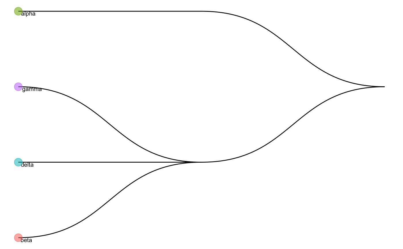
We can also visualise the cell type tree of the reference data.

plotCellTypeTree(cellTypeTree(trainClassExample_xin))

Running scClassify

Next, we perform predict_scClassify with our pretrained model trainRes = trainClassExample to predict the cell types of our query data matrix exprsMat_wang_subset_sparse. Here, we used pearson and spearman as similarity metrics.

pred_res <- predict_scClassify(exprsMat_test = exprsMat_wang_subset,
                               trainRes = trainClassExample_xin,
                               cellTypes_test = wang_cellTypes,
                               algorithm = "WKNN",
                               features = c("limma"),
                               similarity = c("pearson", "spearman"),
                               prob_threshold = 0.7,
                               verbose = TRUE)
#> Performing unweighted ensemble learning... 
#> Using parameters: 
#> similarity  algorithm   features 
#>  "pearson"     "WKNN"    "limma" 
#> [1] "Using dynamic correlation cutoff..."
#> [1] "Using dynamic correlation cutoff..."
#> classify_res
#>                correct   correctly unassigned           intermediate 
#>            0.704590818            0.239520958            0.000000000 
#> incorrectly unassigned         error assigned          misclassified 
#>            0.000000000            0.051896208            0.003992016 
#> Using parameters: 
#> similarity  algorithm   features 
#> "spearman"     "WKNN"    "limma" 
#> [1] "Using dynamic correlation cutoff..."
#> [1] "Using dynamic correlation cutoff..."
#> classify_res
#>                correct   correctly unassigned           intermediate 
#>            0.702594810            0.013972056            0.000000000 
#> incorrectly unassigned         error assigned          misclassified 
#>            0.001996008            0.277445110            0.003992016 
#> weights for each base method: 
#> numeric(0)

Noted that the cellType_test is not a required input. For datasets with unknown labels, users can simply leave it as cellType_test = NULL.

Prediction results for pearson as the similarity metric:

table(pred_res$pearson_WKNN_limma$predRes, wang_cellTypes)
#>                   wang_cellTypes
#>                    acinar alpha beta delta ductal gamma stellate
#>   alpha                 0   206    0     0      0     2        0
#>   beta                  0     0  118     0      1     0        0
#>   beta_delta_gamma      0     0    0     0     25     0        0
#>   delta                 0     0    0    10      0     0        0
#>   gamma                 0     0    0     0      0    19        0
#>   unassigned            5     0    0     0     70     0       45

Prediction results for spearman as the similarity metric:

table(pred_res$spearman_WKNN_limma$predRes, wang_cellTypes)
#>                   wang_cellTypes
#>                    acinar alpha beta delta ductal gamma stellate
#>   alpha                 0   206    0     0      0     2        2
#>   beta                  2     0  118     0     29     0        6
#>   beta_delta_gamma      1     0    0     0     66     0       31
#>   delta                 0     0    0    10      0     0        2
#>   gamma                 0     0    0     0      0    18        0
#>   unassigned            2     0    0     0      1     1        4

Session Info

sessionInfo()
#> R Under development (unstable) (2020-03-25 r78063)
#> Platform: x86_64-apple-darwin15.6.0 (64-bit)
#> Running under: macOS Catalina 10.15.4
#> 
#> Matrix products: default
#> BLAS:   /Library/Frameworks/R.framework/Versions/4.0/Resources/lib/libRblas.0.dylib
#> LAPACK: /Library/Frameworks/R.framework/Versions/4.0/Resources/lib/libRlapack.dylib
#> 
#> locale:
#> [1] en_AU.UTF-8/en_AU.UTF-8/en_AU.UTF-8/C/en_AU.UTF-8/en_AU.UTF-8
#> 
#> attached base packages:
#> [1] stats     graphics  grDevices utils     datasets  methods   base     
#> 
#> other attached packages:
#> [1] scClassify_0.99.2 BiocStyle_2.15.6 
#> 
#> loaded via a namespace (and not attached):
#>  [1] Biobase_2.47.3      viridis_0.5.1       mixtools_1.2.0     
#>  [4] tidyr_1.0.2         tidygraph_1.1.2     viridisLite_0.3.0  
#>  [7] splines_4.0.0       ggraph_2.0.2        RcppParallel_5.0.0 
#> [10] assertthat_0.2.1    statmod_1.4.34      BiocManager_1.30.10
#> [13] stats4_4.0.0        yaml_2.2.1          ggrepel_0.8.2      
#> [16] pillar_1.4.3        backports_1.1.6     lattice_0.20-41    
#> [19] glue_1.4.0          limma_3.43.5        digest_0.6.25      
#> [22] polyclip_1.10-0     colorspace_1.4-1    htmltools_0.4.0    
#> [25] Matrix_1.2-18       pkgconfig_2.0.3     bookdown_0.18      
#> [28] purrr_0.3.3         scales_1.1.0        tweenr_1.0.1       
#> [31] hopach_2.47.0       BiocParallel_1.21.2 ggforce_0.3.1      
#> [34] proxy_0.4-23        tibble_3.0.0        mgcv_1.8-31        
#> [37] farver_2.0.3        ggplot2_3.3.0       ellipsis_0.3.0     
#> [40] BiocGenerics_0.33.3 cli_2.0.2           survival_3.1-12    
#> [43] magrittr_1.5        crayon_1.3.4        memoise_1.1.0      
#> [46] evaluate_0.14       fs_1.4.1            fansi_0.4.1        
#> [49] nlme_3.1-145        MASS_7.3-51.5       segmented_1.1-0    
#> [52] tools_4.0.0         minpack.lm_1.2-1    lifecycle_0.2.0    
#> [55] stringr_1.4.0       kernlab_0.9-29      S4Vectors_0.25.15  
#> [58] munsell_0.5.0       cluster_2.1.0       compiler_4.0.0     
#> [61] pkgdown_1.5.1.9000  proxyC_0.1.5        rlang_0.4.5        
#> [64] grid_4.0.0          rstudioapi_0.11     igraph_1.2.5       
#> [67] labeling_0.3        rmarkdown_2.1       gtable_0.3.0       
#> [70] graphlayouts_0.6.0  R6_2.4.1            gridExtra_2.3      
#> [73] knitr_1.28          dplyr_0.8.5         rprojroot_1.3-2    
#> [76] desc_1.2.0          stringi_1.4.6       parallel_4.0.0     
#> [79] Rcpp_1.0.4.6        vctrs_0.2.4         diptest_0.75-7     
#> [82] tidyselect_1.0.0    xfun_0.12

Performing scClassify using pretrained model

Yingxin Lin

22 April 2020

Introduction

Setting up the data

Running scClassify

Session Info